|
Size: 22668
Comment:
|
← Revision 118 as of 2023-07-17 02:37:25 ⇥
Size: 22648
Comment:
|
| Deletions are marked like this. | Additions are marked like this. |
| Line 11: | Line 11: |
| export SUBJECTS_DIR=$TUTORIAL_DATA/diffusion_tutorial/diffusion_recons cd $TUTORIAL_DATA/diffusion_tutorial |
export SUBJECTS_DIR=$TUTORIAL_DATA/tracula_tutorial/fs cd $TUTORIAL_DATA/tracula_tutorial |
| Line 187: | Line 187: |
| trac-all -stat -c $TUTORIAL_DATA/diffusion_tutorial/dmrirc.tutorial | trac-all -stat -c $TUTORIAL_DATA/tracula_tutorial/dmrirc.tutorial |
Back to list of all tutorials | Back to course page | Previous
Contents
Tract statistics
Remember...
For each new terminal that you open, you must do:
export SUBJECTS_DIR=$TUTORIAL_DATA/tracula_tutorial/fs cd $TUTORIAL_DATA/tracula_tutorial
This section of the tutorial will teach you how to extract statistics on anisotropy and diffusivity measures for the white-matter pathways reconstructed by TRACULA. There are two types of statistics files that are created for each white-matter pathway:
pathstats.overall.txt - This file contains diffusion measures averaged over the whole pathway.
pathstats.byvoxel.txt - This file contains diffusion measures averaged at consecutive cross-sections of the pathway, resulting in an along-tract profile of each diffusion measure. This type of analysis is referred to as pointwise assessment of streamline tractography attributes (PASTA).
These are plain text files that you can open with a text editor, such as gedit on Linux, or with the command open -e on a Mac. They are saved in the TRACULA output directory of each individual tract.
Anisotropy and diffusivity averaged over an entire pathway
Examine the whole-tract statistics for the left inferior longitudinal fasciculus (ILF) of subject1, by runnning:
cat trc/subject1/dpath/lh.ilf_avg16_syn_bbr/pathstats.overall.txt
This file will look like this:
# Title Pathway Statistics
#
# generating_program /usr/local/freesurfer/7.2.0-beta/bin/dmri_pathstats
# cvs_version ayendiki-local
# cmdline /usr/local/freesurfer/7.2.0-beta/bin/dmri_pathstats --intrc /space/erebus/1/users/data/trc/subject1/dpath/lh.ilf_avg16_syn_bbr --dtbase /space/erebus/1/users/data/trc/subject1/dmri/dtifit --path lh.ilf --subj subject1 --invox path.ref.txt --out /space/erebus/1/users/data/trc/subject1/dpath/lh.ilf_avg16_syn_bbr/pathstats.overall.txt --outvox /space/erebus/1/users/data/trc/subject1/dpath/lh.ilf_avg16_syn_bbr/pathstats.byvoxel.txt
# sysname Linux
# hostname compute-0-124.nmr.mgh.harvard.edu
# machine x86_64
# user ayendiki
# anatomy_type pathway
#
# subjectname subject1
# pathwayname lh.ilf
#
Count 1500
Volume 1996
Len_Min 53
Len_Max 129
Len_Avg 79.9787
Len_Center 89
AD_Avg 0.00120044
AD_Avg_Weight 0.00121209
AD_Avg_Center 0.00123318
RD_Avg 0.000467543
RD_Avg_Weight 0.000458132
RD_Avg_Center 0.000549716
MD_Avg 0.000711842
MD_Avg_Weight 0.000709453
MD_Avg_Center 0.000777538
FA_Avg 0.540167
FA_Avg_Weight 0.553683
FA_Avg_Center 0.477498
This text file contains various diffusion measures, averaged over the entire pathway (in this example, the left ILF). The measures include:
- Number of sample paths drawn from the probability distribution of the pathway (Count)
- Volume of the probability distribution of the pathway (in voxels)
- Maximum, minimum, and average length of the sample paths (in voxels)
- Length of the highest-probability (a.k.a. maximum a posteriori) path
- Axial diffusivity (average over the entire support of the path distribution, weighted average over the entire support of the path distribution, and average over highest-probability path only)
- Radial diffusivity (as above)
- Mean diffusivity (as above)
- Fractional anisotropy (as above)
Combining pathstats.overall.txt files for group analyses
Measures can be extracted from these files and concatenated across subjects, e.g., for group analysis. Specifically, the text files can be converted into a table using the command tractstats2table and then used for doing GLM analyses with mri_glmfit or any other statistical software (SPSS, Excel, Statview etc.)
Before using tractstats2table, you have to create a text file that lists the full path to the pathstats.overall.txt files from all subjects that you want to include in your analysis. For example, if you wanted to analyze whole-tract measures from the left ILF of 3 subjects, you would create a text file that looks like the following:
$TUTORIAL_DATA/diffusion_tutorial/trc/subject1/dpath/lh.ilf_avg16_syn_bbr/pathstats.overall.txt
$TUTORIAL_DATA/diffusion_tutorial/trc/subject2/dpath/lh.ilf_avg16_syn_bbr/pathstats.overall.txt
$TUTORIAL_DATA/diffusion_tutorial/trc/subject3/dpath/lh.ilf_avg16_syn_bbr/pathstats.overall.txt
Create a text file called lh.ilf.list using the command below. Copy and paste the list above into this file, then save the file and exit the editor.
gedit lh.ilf.list &
ON MACS, RUN:
open -e lh.ilf.list &
The following command will use this list to create a table with the diffusion measures from all the subjects listed above:
tractstats2table --load-pathstats-from-file lh.ilf.list --overall --tablefile lh.ilf.All.table
The argument to the --load-pathstats-from-file option specifies the text file that contains the list of all the statistics files that will be combined.
Take a look at the resulting table file:
gedit lh.ilf.All.table &
ON MACS, RUN:
open -e h.ilf.All.table &
Instead of extracting all measures included in the pathstats.overall.txt files, we are usually interested only in a few specific measures. For example, to extract only the average FA for each subject, do the following:
tractstats2table --load-pathstats-from-file $lh.ilf.list --overall --only-measures FA_Avg --tablefile lh.ilf.FA_Avg.table
The argument to the --only-measures option specifies which measure we want to extract from the statistics files. Instead of FA_Avg, this could be the name of any of the measures included in pathstats.overall.txt.
OPTIONAL: You can look at these tables in OpenOffice (or any other spreadsheet program). For example, to open the file lh.ilf.FA_Avg.table in OpenOffice, do the following :
localc lh.ilf.FA_Avg.table
You can then use these stats tables as input to mri_glmfit, to run perform group analysis.
Fitting a general linear model to whole-tract measures
In this scenario, we are treating each tract as a single region of interest, so we have one value of the measure of interest (e.g., average FA) for each tract. In this sense, performing statistics on the average FA of the left ILF is similar to performing statistics, e.g., the volume of the thalamus or the average thickness of the superior frontal cortex. You can do this as follows:
mri_glmfit --table lh.ilf.FA_Avg.table \
           --fsgd age-sex.fsgd dods \
           --C age-slope-female-v-male.mtx \
           --o lh.ilf.FA_Avg.glmdir
--table: Any stats table created by tractstats2table
--fsgd: A FreeSurfer group descriptor (FSGD) file, which contains a list of all subjects and all continuous or discrete variables (e.g., sex, age, motion, etc.) that you want to include in the model. Alternatively, --X can be used to specify the design matrix instead of an FSGD file. For more information on how to set up the FSGD file, see the Design Matrix/FSGD File section of the FreeSurfer group analysis tutorial.
--C: A contrast matrix that defines the hypothesis that you want to test, e.g., a difference in the slope of average FA vs. age between female and male subjects. For more information on how to set up the contrast matrix, see the Contrasts section of the FreeSurfer group analysis tutorial.
--o: The name of the output directory where the results of the statistical analysis will be saved. For more information on the files that mri_glmfit saves in its output directory, see the GLM Analysis section of the FreeSurfer group analysis tutorial.
Anisotropy and diffusivity averaged at cross-sections along a pathway
Now examine the along-tract (PASTA) statistics for the right uncinate fasciculus (UF), by running:
cat trc/subject1/dpath/rh.uf_avg16_syn_bbr/pathstats.byvoxel.txt
# Title Pathway Statistics
#
# generating_program /usr/local/freesurfer/7.2.0-beta/bin/dmri_pathstats
# cvs_version ayendiki-local
# cmdline /usr/local/freesurfer/7.2.0-beta/bin/dmri_pathstats --intrc /space/erebus/1/users/data/trc/subject1/dpath/rh.uf_avg16_syn_bbr --dtbase /space/erebus/1/users/data/trc/subject1/dmri/dtifit --path rh.uf --subj subject1 --invox path.ref.txt --out /space/erebus/1/users/data/trc/BANDA001/dpath/rh.uf_avg16_syn_bbr/pathstats.overall.txt --outvox /space/erebus/1/users/data/trc/subject1/dpath/rh.uf_avg16_syn_bbr/pathstats.byvoxel.txt
# sysname Linux
# hostname compute-0-124.nmr.mgh.harvard.edu
# machine x86_64
# user ayendiki
# anatomy_type pathway
#
# subjectname subject1
# pathwayname rh.uf
#
# pathway start
x y z AD RD MD FA AD_Avg RD_Avg MD_Avg FA_Avg
63 114 16 0.000903693 0.00073526 0.000791404 0.128285 0.00106562 0.000548642 0.000720969 0.419023
62 114 17 0.000997801 0.00061554 0.000742961 0.292562 0.00106592 0.000548794 0.00072117 0.418772
62 113 18 0.000979601 0.000629353 0.000746102 0.27799 0.00109077 0.000540408 0.000723864 0.436669
63 112 18 0.00092282 0.000642831 0.000736161 0.268556 0.00110944 0.0005337 0.000725612 0.450405
63 111 18 0.000874507 0.000687739 0.000749995 0.161811 0.00112578 0.000534306 0.000731465 0.455462
...
49 81 14 0.00117395 0.000526631 0.000742404 0.471764 0.00117598 0.000556707 0.00076313 0.442443
49 82 13 0.000971424 0.000614876 0.000733725 0.328818 0.00116098 0.000564635 0.000763416 0.429103
49 82 13 0.000971424 0.000614876 0.000733725 0.328818 0.00116098 0.000564635 0.000763416 0.429103
49 83 12 0.00113972 0.000584445 0.000769535 0.41186 0.00113818 0.000577262 0.000764234 0.408795
49 84 12 0.00130902 0.000540453 0.000796644 0.511488 0.00112725 0.000584374 0.000765331 0.39815
# pathway end
This text file contains various diffusion measures, one row for each position along the trajectory of the path. The first three entries in each row are the x, y, z coordinates in native diffusion space. The next four entries are the axial diffusivity, radial diffusivity, mean diffusivity, and fractional anisotropy at that position on the maximum a posteriori path. The last four entries are the axial diffusivity, radial diffusivity, mean diffusivity, and fractional anisotropy at the same position, averaged over all sampled paths.
Points are ordered according to the following convention (see also along-tract plots):
- For pathways with a right-left orientation:
- If the pathway is inter-hemispheric: From right to left
- If the pathway is intra-hemispheric: From medial to lateral
- For pathways with an anterior-posterior orientation: From anterior to posterior
- For pathways with a superior-inferior orientation: From superior to inferior
Combining pathstats.byvoxel.txt files for group analyses
You can combine the pathstats.byvoxel.txt files from multiple subjects, to use as input for along-tract group analysis, by running the following:
trac-all -stat -c $TUTORIAL_DATA/tracula_tutorial/dmrirc.tutorial
This will create a directory named stats under the main TRACULA output directory. For each tract and each diffusion measure, TRACULA saves the table of concatenated along-tract profiles both as a text file, where each row is a different position along the tract and each column is a different subject, and as a NIfTI volume. For group analyses, you can either pass the NIfTI table to mri_glmfit (see below), or import the text table to the statistical analysis package of your choice.
To examine the text table of average RD values along the right UF, do the following:
gedit trc/stats/rh.uf.avg16_syn_bbr.RD_Avg.txt &
ON MACS, RUN:
open -e trc/stats/rh.uf.avg16_syn_bbr.RD_Avg.txt &
The contents of this file will look like this:
subject1 subject2 subject3
0.000548642 0.000544788 0.000524961
0.000548794 0.00054724 0.000523532
0.000540408 0.000537787 0.000512756
0.0005337 0.000529497 0.000508355
0.000534306 0.000529497 0.000508355
0.000527594 0.000523291 0.000504756
0.000522767 0.000519212 0.000509367
0.000521042 0.000511412 0.000506172
0.000505337 0.000515574 0.000511211
0.000484886 0.000515537 0.000513693
...
The first row tells you the subject names for the corresponding columns of along-tract RD values.
To examine the NIfTI table of average RD values along the right UF, do the following:
mri_info trc/stats/rh.uf.avg16_syn_bbr.FA_Avg.nii.gz &
From the output of mri_info, you can see that the size of the first dimension of this volume is the number of points along the tract (here 72), and the size of the last dimension is the number of subjects (here 3). The voxel sizes show the distance between consecutive position along the tract where the diffusion measures are sampled.
          type: nii
    dimensions: 72 x 1 x 1 x 3
   voxel sizes: 1.500000, 1.500000, 1.500000
          type: FLOAT (3)
...
Fitting a general linear model to along-tract measures
In this scenario, we have a series of values for the measure of interest (e.g., the RD) along each tract. Performing statistics on the values that RD takes at different points along the right UF is similar to performing statistics, e.g., on the values that cortical thickness takes along the cortical surface, in the sense that we have to account for the multiple comparisons. The main difference here is that, whereas surface-based analyses are done in 2D, along-tract analyses are done in 1D (because we are looking at a series of cross-sections of the tract) and involve far fewer comparisons.
First, you can fit a general linear model (GLM) at each point along the tract, and obtain uncorrected statistics, as follows:
mri_glmfit --y trc/stats/rh.uf.avg16_syn_bbr.RD_Avg.nii.gz \
           --fsgd age-sex.fsgd dods \
           --C age-slope-female-v-male.mtx \
           --o rh.uf.RD_Avg.glmdir --save-eres
--y: Any of the along-tract stats volumes produced by trac-all --stat.
--fsgd: A FreeSurfer group descriptor (FSGD) file, which contains a list of all subjects and all continuous or discrete variables (e.g., sex, age, motion, etc.) that you want to include in the model. Alternatively, --X can be used to specify the design matrix instead of an FSGD file. For more information on how to set up the FSGD file, see the Design Matrix/FSGD File section of the FreeSurfer group analysis tutorial.
--C: A contrast matrix that defines the hypothesis that you want to test, e.g., a difference in the slope of average RD vs. age between female and male subjects. For more information on how to set up the contrast matrix, see the Contrasts section of the FreeSurfer group analysis tutorial.
--o: The name of the output directory where the results of the statistical analysis will be saved. For more information on the files that mri_glmfit saves in its output directory, see the GLM Analysis section of the FreeSurfer group analysis tutorial.
Pro tip: By default, mri_glmfit saves any of its outputs that are volumes in .mgh format. You can change this behavior by using, e.g., --mgz or --nii or --nii.gz. If you want to convert any of these volumes to a text file (e.g., to read the p-values along the tract into your own script for further processing), you can use, for example, mri_convert --ascii sig.mgh sig.txt.
After running mri_glmfit, you can perform cluster-wise correction for multiple comparisons on its outputs as follows:
mri_glmfit-sim --glmdir rh.uf.RD_Avg.glmdir \
               --cwp .05 \
               --perm 1000 1.3 pos
--glmdir: The output directory of the mri_glmfit command above
--cwp thresh: The cluster-wise threshold for statistical significance. In the example above, we are keeping only clusters that have cluster-wise p-values < 0.05. To keep all clusters, set this to .999.
--perm niter thresh sign: Settings for permutation simulation. In the example above, we are running 1000 iterations, we are using a cluster-forming threshold of 1.3 (meaning -log10(p) = 1.3), and we are testing for a positive contrast (the sign can be: pos, neg, abs).
For more information on mri_glmfit-sim and its outputs, see the Clusterwise Correction for Multiple Comparisons section of the FreeSurfer group analysis tutorial. In the previous example, the output files will be named perm.th13.pos.sig.*, e.g., the list of significant clusters will be in a file called perm.th13.pos.sig.cluster.summary.
Visualizing results from statistical analyses along a pathway
By default, TRACULA uses the mean of its manually annotated training streamlines to determine the positions along each of the 42 pathways where diffusion measures will be projected. These mean streamlines are saved in template space (the template that is the target of the inter-subject registration) and mapped to each individual subject after the individual subject's pathways are reconstructed, to extract the along-tract measures. Note that these mean paths are only used to determine how each pathway will be sliced up into into cross-sections where along-tract measures will be averaged, and to ensure an equal number of cross-sections for all subjects.
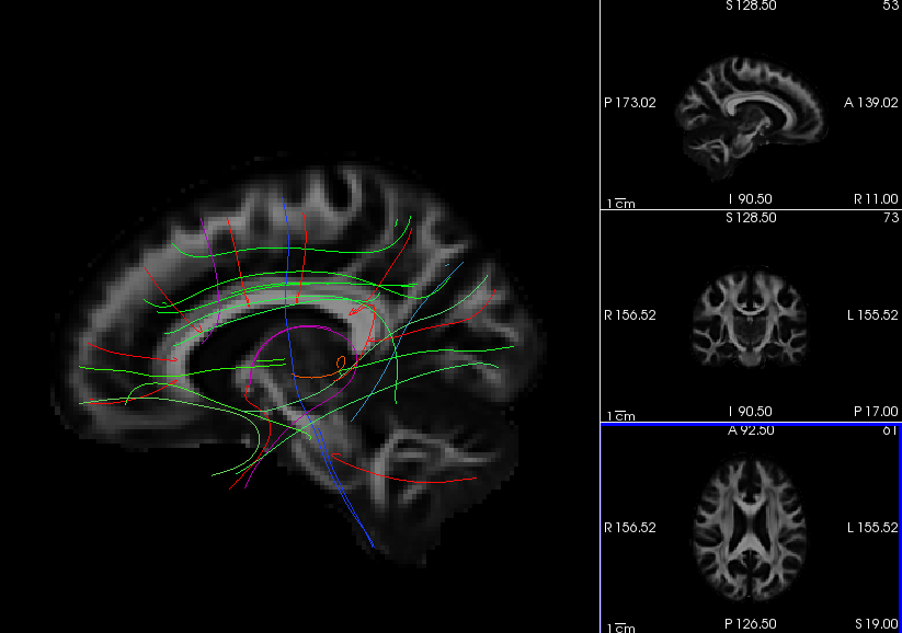
To view all 42 mean paths in template space, run the following:
freeview -v $FREESURFER_HOME/trctrain/hcp/MGH35_HCP_FA_template.nii.gz \
         -t $FREESURFER_HOME/trctrain/hcp/syn/*.mean.trk
You should see something like this in the 3D view:

In addition, a subset of the training streamlines from each pathway have been saved in a .trk file in template space, which can be used to overlay the outputs of along-tract statistical analysis and visualize them in freeview.
Let's assume that you have used mri_glmfit to perform along-tract statistical analysis of the average radial diffusivity (RD) along the left and right uncinate fasciculus (UF), and that you saved the outputs in the directories trc/stats/glmdir.lh.uf.RD_Avg and trc/stats/glmdir.rh.uf.RD_Avg. You can embed any of the *.mgh statistical maps that were output by mri_glmfit into the template .trk files for left and right UF using the dmri_trk2trk command. This will allow you to then visualize these statistical maps along the tracts in freeview.
For example, let's embed the sig.mgh and z.mgh maps from the analysis of average RD along the left UF into the template .trk file for the left UF:
dmri_trk2trk --in $FREESURFER_HOME/trctrain/hcp/syn/lh.uf.display.trk \
             --out trc/stats/lh.uf.overlay.trk \
             --over trc/stats/lh.uf.RD_Avg.glmdir/contrast1/sig.mgh \
                    trc/stats/lh.uf.RD_Avg.glmdir/contrast1/z.mgh
Next, we'll do the same for the right UF:
dmri_trk2trk --in $FREESURFER_HOME/trctrain/hcp/syn/rh.uf.display.trk \
             --out trc/stats/rh.uf.overlay.trk \
             --over trc/stats/rh.uf.RD_Avg.glmdir/contrast1/sig.mgh \
                    trc/stats/rh.uf.RD_Avg.glmdir/contrast1/z.mgh
We will now display the .trk files that we created over the template brain:
freeview -v $FREESURFER_HOME/trctrain/hcp/MGH35_HCP_FA_template.nii.gz \
         -t trc/stats/lh.uf.overlay.trk trc/stats/rh.uf.overlay.trk
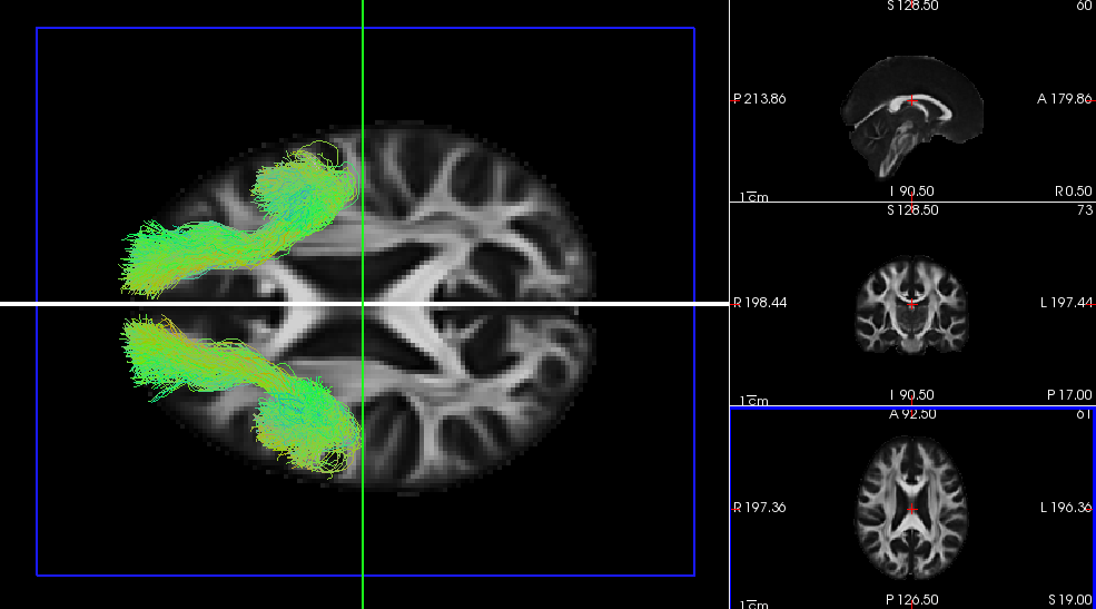
When we first open freeview, the streamlines from the .trk files are displayed in their usual directional colormap (so they are green, as the UF runs mostly anterior-posterior):

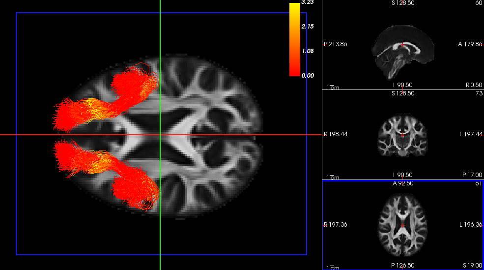
However, because we embeded the values of the along-tract statistical maps in these .trk files, we can now choose to use one of those statistical maps as the colormap for the corresponding tract.
- Select one of the .trk files (lh.uf or rh.uf) from the panel in the top left of the freeview window.
From the Color code menu on the left, choose Scalar.
From the Scalar menu, you can select either of the two statistical maps that you embeded in this .trk file: sig.mgh or z.mgh
From the Color menu, you can select the colormap for the statistical map. By default, it is set to Heatscale and you can change the Min and Max of the heatscale from the sliders below.
- Click on the colorbar button on the top bar of the freeview window to display a colorbar for this heatscale.
Repeat this for both the left and right UF. The end result will look something like this in the 3D view:

Summary
By the end of this page, you should know how to:
- Extract statistics (anisotropy and diffusivity measures), either averaged over an entire white-matter pathway, or averaged at different positions along a pathway
- Combine statistics into tables for group analysis
- Perform whole-tract and along-tract statistical analysis
- Visualize the outputs of along-tract statistical analysis in freeview
Quiz
You can test your knowledge of this tutorial by clicking here for a quiz!
Back to list of all tutorials | Back to course page | Previous
