|
Size: 2471
Comment: changed from WorkFlowTemplate to headings
|
Size: 6506
Comment: overlays should be written as .mgh, not .w files
|
| Deletions are marked like this. | Additions are marked like this. |
| Line 1: | Line 1: |
| ## Note that the use of 2 commas is not a typo. | ||Up to TkSurferGuide||Back to [[../TkSurferCurvature| TkSurferCurvature]]||Continue to [[../TkSurferTimeCourse| TkSurferTimeCourse]]|| |
| Line 3: | Line 3: |
| == Overlay == | = Overlay = |
| Line 5: | Line 5: |
| An overlay is a set of values, 0 or 1 per vertex, displayed with a color scale. It is normally used as a functional activation overlay, but can really be any floating point value per voxel. The source volume can be a .w file, a file containing one value per vertex, previously registered with the volume. It can also be a binary volume or bfile. These are volumes of short integers (.bshort) or floating point values (.bfloat) with a corresponding registration file. Binary volumes can contain multiple time points and conditions. | An overlay is a set of values for vertices displayed on top of the surface with a color scale. It is normally used as a functional activation overlay, but can really be any floating point value per voxel. |
| Line 7: | Line 7: |
| Overlays can be loaded into any of five layers. TkSurfer can display one overlay layer at a time. | The source data can be a .w file, which is a file of scalar values associated with vertex indices. This data is associated by vertex index, so needs no additional registration. It's just painted right onto the surface, which is why it's sometimes called a paint file. |
| Line 9: | Line 9: |
| === Loading Overlay Files === | The source data can also be a volume. In this case, the surface is intersected with the volume in real space, so the volume needs to be registered to the surface somehow. Volumes can have more than one frame of data, which translates into time points. Additionally, some volume types have header data which describe how additional frames should be interpreted as time points or conditions, such as output from the fsfast stream. |
| Line 11: | Line 11: |
| To load an overlay file, use the '''File->Load Overlay...''' item. You will be prompted for the overlay file name and the layer in which to load the file. Chose the .w file or a .bshort or .bfloat file if you are loading a binary volume. | TkSurfer can load up to eight overlays, although it can only display one overlay layer at a time. |
| Line 13: | Line 13: |
| If you are loading a binary volume, you will be prompted for the stem of the volume and a registration file. You may leave the registration file field blank if there is a registration file in the same directory as the binary volume named "register.dat." | == Loading Overlay Files == |
| Line 15: | Line 15: |
| === Overlay File Display Options === | To load an overlay file, use the '''File->Load Overlay...''' item or control-right click the overlay button in the toolbar. You will be prompted for the overlay file name and the layer in which to load the file. Specify a .w file (deprecated) or a .mgh volume file. If you specify a volume, you must also choose a registration method (if you are loading a .w file, ignore the registration type). These are the options: |
| Line 17: | Line 17: |
| To select which overlay to show, use the '''View->Overlay Layer''' submenu. The field names are automatically set to the file name loaded. You can change this name by typing a new one into the information area in the Tool window. | ||Specify registration file||If you have a register.dat file, probably generated by TkRegister, use this option to specify it. The file contains a transformation matrix, some information about voxel size, and a rounding method.|| ||Find registration in data directory||If you have a register.dat file in the same directory as the data file, use this option to automatically look in that directory.|| ||Calculate identity matrix||If the functional volume is in the same alignment as the anatomical volume, or you do not wish to register the functional volume, use this option. It will calculate a proper "identity" matrix based on the parameters of the functional and anatomical volumes. Note that an orig volume must be present for the subject you are loading for this method to work.|| |
| Line 19: | Line 21: |
| The display for the current overlay can be configured in the '''View->Configure->Configure Overlay Display''' dialog. If the data you have loaded has multiple time points or conditions, you can select which one to show with the '''Time Point''' and '''Condition''' fields. You can select the color scale to use with the radio buttons in the top area of the dialog. The '''Truncate''' option can be checked to turn off the display of negative values. Check the '''Reverse''' option to reverse the sign of the values as they are drawn in the color scale. '''Inverse and Complex are reserved for future upgrades.''' Also see SettingTheOverlayColorScale. | == Overlay File Display Options == To select which overlay to show, use the '''View->Overlay Layer''' submenu or click the * button to the right of the overlay label in the information area of the tools window. The field names are automatically set to the file name loaded. You can change this name by typing a new one into the information area in the Tool window. The display for the current overlay can be configured in the '''View->Configure->Configure Overlay Display''' dialog. Here are the options: '''Opacity:''' This is the opacity of the overlay data. '''Location:''' If the data you have loaded has multiple time points or conditions, you can select which one to show with the '''Time Point''' and '''Condition''' fields. '''Color scale:''' This simply chooses a color scale with which to display the data. Curvature usually uses green/red, functional data usually uses heat scale, and field sign data usually uses blue/red. '''Truncate:''' If checked, this will turn off the display of negative values. '''Inverse:''' If checked, this will reverse the sign of the values as they are drawn in the color scale. '''Complex:''' If checked, interprets the data as complex values. '''Ignore Zeroes in Histogram:''' If checked, zero values will not be shown in the histogram. If the overlay is sparse and has few non-zero values, this can save a tall spike of zero values in the histogram that makes it hard to see other values. '''Threshold type:''' In Linear mode, the color map is a linear scale from min to max (see below). Values below min will not be displayed, the value of min will be dark red, the value of max will be yellow, and all values above max will be yellow. In Piecewise mode, two linear scales are used: one from min to mid, and another from mid to max. You can also set the second linear scale using a slope instead of specifying a max. '''Threshold minimum / midpoint / maximum / slope:''' Use these values to set up the linear or piecewise threshold scale. To set the values, enter a value in a field, and press return. Then click the Apply button to use the new scale. When setting the max or slope, pressing return when setting one value will update the other value accordingly. You can configure the thresholds either by entering values into the labeled fields, or by clicking on the histogram. To set using the histogram, click with the left button to set the Min threshold, the middle button for the Mid threshold, and the right button for the Max threshold. When you click the Apply button, the colors of the value bars in the histogram will change to reflect the new color scale. Note how the threshold bars on both the positive and negative sides of the histogram update. '''The Offset field''', primarily, shifts the axis to the offset value horizontally. After you enter a non-zero offset in the textbox, all actions pertaining to the histogram from thereon are relative to the offset. The lines are now symmetric to offset value rather than 0 point. The Min, (Mid) and Max text entry boxes show values which are relative to the offset and the values you enter in the boxes are relative as well. To get back to normal settings, enter 0.0 in the Offset field. '''Copy Settings to Layer:''' Choose a layer and click this button to copy the layer settings to another layer. '''Apply changes to all layers:''' If this is checked, clicking Apply will apply your changes to all layers, changing the settings of all layers to the current values. '''Set Threshold Using FDR:''' This will automatically set the threshold values using False Rate Discovery. Enter the rate in the field next to the button. If the Only Marked checkbox is checked, only values that are marked will be considered. |
| Line 23: | Line 57: |
| === Saving Overlay Files === | == Saving Overlay Files == |
| Line 25: | Line 59: |
| An overlay can only be written out to a .w file; binary volumes cannot be written from overlays. To write a .w file, choose '''File->Save Overlay As...''', and choose a file name and layer from the dialog box. | An overlay should be written out to a .mgh file; binary volumes cannot be written from overlays. To write a .mgh file, choose '''File->Save Overlay As...''', and choose a file name and layer from the dialog box. |
| Line 31: | Line 65: |
Up to TkSurferGuide |
Back to TkSurferCurvature |
Continue to TkSurferTimeCourse |
Overlay
An overlay is a set of values for vertices displayed on top of the surface with a color scale. It is normally used as a functional activation overlay, but can really be any floating point value per voxel.
The source data can be a .w file, which is a file of scalar values associated with vertex indices. This data is associated by vertex index, so needs no additional registration. It's just painted right onto the surface, which is why it's sometimes called a paint file.
The source data can also be a volume. In this case, the surface is intersected with the volume in real space, so the volume needs to be registered to the surface somehow. Volumes can have more than one frame of data, which translates into time points. Additionally, some volume types have header data which describe how additional frames should be interpreted as time points or conditions, such as output from the fsfast stream.
TkSurfer can load up to eight overlays, although it can only display one overlay layer at a time.
Loading Overlay Files
To load an overlay file, use the File->Load Overlay... item or control-right click the overlay button in the toolbar. You will be prompted for the overlay file name and the layer in which to load the file. Specify a .w file (deprecated) or a .mgh volume file. If you specify a volume, you must also choose a registration method (if you are loading a .w file, ignore the registration type). These are the options:
Specify registration file |
If you have a register.dat file, probably generated by TkRegister, use this option to specify it. The file contains a transformation matrix, some information about voxel size, and a rounding method. |
Find registration in data directory |
If you have a register.dat file in the same directory as the data file, use this option to automatically look in that directory. |
Calculate identity matrix |
If the functional volume is in the same alignment as the anatomical volume, or you do not wish to register the functional volume, use this option. It will calculate a proper "identity" matrix based on the parameters of the functional and anatomical volumes. Note that an orig volume must be present for the subject you are loading for this method to work. |
Overlay File Display Options
To select which overlay to show, use the View->Overlay Layer submenu or click the * button to the right of the overlay label in the information area of the tools window. The field names are automatically set to the file name loaded. You can change this name by typing a new one into the information area in the Tool window.
The display for the current overlay can be configured in the View->Configure->Configure Overlay Display dialog. Here are the options:
Opacity: This is the opacity of the overlay data.
Location: If the data you have loaded has multiple time points or conditions, you can select which one to show with the Time Point and Condition fields.
Color scale: This simply chooses a color scale with which to display the data. Curvature usually uses green/red, functional data usually uses heat scale, and field sign data usually uses blue/red.
Truncate: If checked, this will turn off the display of negative values.
Inverse: If checked, this will reverse the sign of the values as they are drawn in the color scale.
Complex: If checked, interprets the data as complex values.
Ignore Zeroes in Histogram: If checked, zero values will not be shown in the histogram. If the overlay is sparse and has few non-zero values, this can save a tall spike of zero values in the histogram that makes it hard to see other values.
Threshold type: In Linear mode, the color map is a linear scale from min to max (see below). Values below min will not be displayed, the value of min will be dark red, the value of max will be yellow, and all values above max will be yellow. In Piecewise mode, two linear scales are used: one from min to mid, and another from mid to max. You can also set the second linear scale using a slope instead of specifying a max.
Threshold minimum / midpoint / maximum / slope: Use these values to set up the linear or piecewise threshold scale. To set the values, enter a value in a field, and press return. Then click the Apply button to use the new scale. When setting the max or slope, pressing return when setting one value will update the other value accordingly. You can configure the thresholds either by entering values into the labeled fields, or by clicking on the histogram. To set using the histogram, click with the left button to set the Min threshold, the middle button for the Mid threshold, and the right button for the Max threshold. When you click the Apply button, the colors of the value bars in the histogram will change to reflect the new color scale. Note how the threshold bars on both the positive and negative sides of the histogram update.
The Offset field, primarily, shifts the axis to the offset value horizontally. After you enter a non-zero offset in the textbox, all actions pertaining to the histogram from thereon are relative to the offset. The lines are now symmetric to offset value rather than 0 point. The Min, (Mid) and Max text entry boxes show values which are relative to the offset and the values you enter in the boxes are relative as well. To get back to normal settings, enter 0.0 in the Offset field.
Copy Settings to Layer: Choose a layer and click this button to copy the layer settings to another layer.
Apply changes to all layers: If this is checked, clicking Apply will apply your changes to all layers, changing the settings of all layers to the current values.
Set Threshold Using FDR: This will automatically set the threshold values using False Rate Discovery. Enter the rate in the field next to the button. If the Only Marked checkbox is checked, only values that are marked will be considered.
Click the Apply button to see your changes.
Saving Overlay Files
An overlay should be written out to a .mgh file; binary volumes cannot be written from overlays. To write a .mgh file, choose File->Save Overlay As..., and choose a file name and layer from the dialog box.