Longitudinal Processing - Tutorial

This page will take you through the steps of processing your longitudinal data:

Contents

Preparations
Longitudinal Image Processing
Inspecting Longitudinal Data
Post-Processing Longitudinal Data
Editing Longitudinal Data

After the tutorial (if you want to learn more) you can read details about the longitudinal stream at LongitudinalProcessing, LongitudinalEdits and LongitudinalStatistics.

1. Preparations

If you are taking one of the formally organized courses, everything has been set up for you on the provided laptop. The only thing you will need to do is run the following commands in every new terminal window (aka shell) you open throughout this tutorial. Copy and paste the commands below to get started:

export SUBJECTS_DIR=$TUTORIAL_DATA/long-tutorial
cd $SUBJECTS_DIR

To copy: Highlight the command in the box above, right click and select copy (or use keyboard shortcut Ctrl+c), then use the middle button of your mouse to click inside the terminal window (this will paste the command). Press enter to run the command.

These two commands set the SUBJECTS_DIR variable to the directory where the data is stored and then navigates into this directory.

If you are NOT taking one of the formally organized courses, click here.

2. Longitudinal Image Processing

All data for this tutorial has already been processed for you (processing can take up to 24h). However, to continue you need to understand the three processing steps (cross, base, long) and associated directory names.

For example, assume you have a subject with two time points: OAS2_0001_MR1 and OAS2_0001_MR2.

[CROSS]: You would process these two images independently first (we call that cross as in crossectional analysis/processing) using the regular freesurfer processing stream (recon-all). You end up with two directories with the names OAS2_0001_MR1 and OAS2_0001_MR2
[BASE]: Then you would run the second step to create the within subject template (also called base) and end up with a new directory. There is only one base directory per subject. We decide to name the base: OAS2_0001. Inside this directory are the results for the average anatomy of your subject across time. You don't use this data in any analysis, and only look at it for quality checking or editing.
[LONG]: Finally you would create the two longitudinal runs (the ones you are actually interested in). You end up with two more directories (these names get automatically assigned): OAS2_0001_MR1.long.OAS2_0001 and OAS2_0001_MR2.long.OAS2_0001. They contain the final, most reliable and accurate processing results.

You can now continue with the next section (inspecting the data).

If you want to learn about the exact commands for processing your data, click here.

3. Inspecting Longitudinal Data

Finally you get to try out a few commands! We use freeview (FreeviewGuide) as a viewer in this tutorial.

First let's check the base (subject template) of a single subject. Open the norm.mgz and surfaces with freeview. If you run the following command and freeview opens in another view, you can click on the Coronal button in order to see the data in the same view:

freeview -v OAS2_0001/mri/norm.mgz \
         -f OAS2_0001/surf/lh.pial:edgecolor=red \
            OAS2_0001/surf/rh.pial:edgecolor=red \
            OAS2_0001/surf/lh.white:edgecolor=blue \
            OAS2_0001/surf/rh.white:edgecolor=blue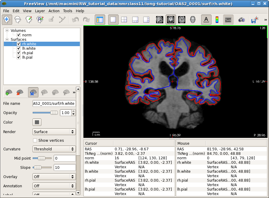

This will show you the within-subject template (base), i.e., the average anatomy of this subject across time overlayed with the pial and white surface. If the across-time registration failed you would see a blurry image or ghosts. You should inspect the surfaces on this image. This will be important later as the surfaces are transferred into the longitudinal runs and therefore should be accurate in the base. Move back and forth a few slices and see if the surfaces follow the white matter and gray matter boundaries.

Now it is time to look at the longitudinal results. Starting with Freesurfer 5.1, the base and the long runs are all in the same voxel space, therefore images across time are already aligned and can be directly compared if opened on top of each other (how convenient ;-). Close any open freeview window to reduce memory usage and run the following command:

freeview -v OAS2_0001_MR1.long.OAS2_0001/mri/norm.mgz \
            OAS2_0001_MR2.long.OAS2_0001/mri/norm.mgz \
         -f OAS2_0001_MR1.long.OAS2_0001/surf/lh.pial:edgecolor=red \
            OAS2_0001_MR1.long.OAS2_0001/surf/lh.white:edgecolor=blue \
            OAS2_0001_MR2.long.OAS2_0001/surf/lh.pial:edgecolor=255,128,128 \
            OAS2_0001_MR2.long.OAS2_0001/surf/lh.white:edgecolor=lightblue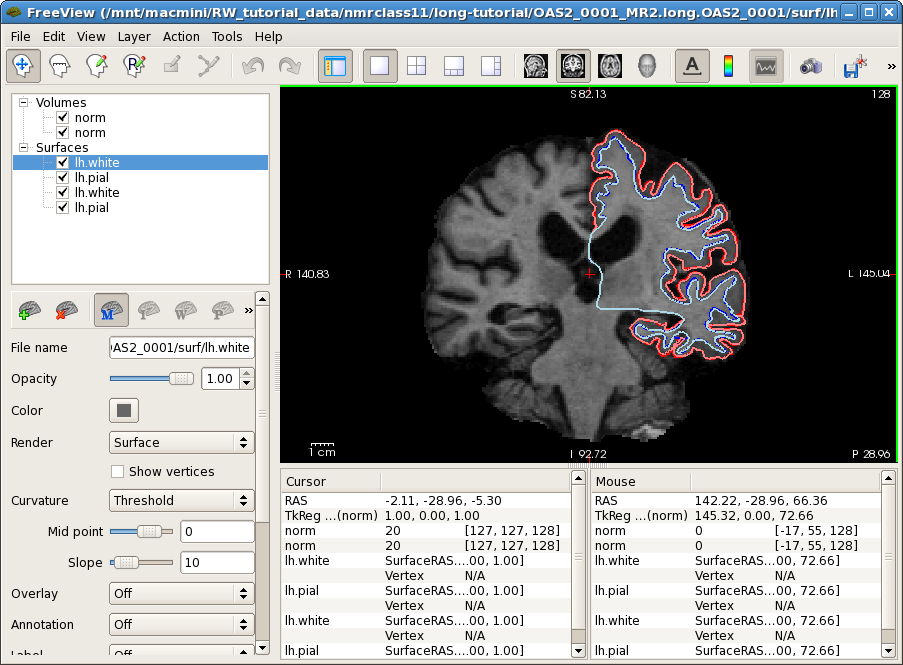

This might take a while to load (check the progress bar). You will see the normalized skull stripped images (norm.mgz) of both time points on top of each other (the second time point is the top-most layer and so the only one visible at the moment). You also see the white and pial surface for each time point, drawn on top of each other (we only show the left hemisphere here to reduce memory usage for older computers). Time point 1 uses red and blue while time point 2 uses pink and light blue for the surface colors. The surfaces do not change much across time. You can also compare the images directly. For this, uncheck the 4 check boxes in front of all the surfaces, or press 'Ctrl-f'. Select the first (top) norm volume and use the opacity slider to blend between the two images. You can also switch back and forth between the two images by pressing 'Alt-c' or using the opacity slider. This way you can spot longitudinal deformations (atrophy) and also potential global alignment problems (not in this case). You will mainly notice that the ventricles are getting larger in the second time point. You can use the Up and Down arrow keys to scroll through the slices.

4. Post-Processing Longitudinal Data

4.1. Longitudinal QDEC Table

(Also: LongitudinalQdecTable)

To get the longitudinal data ready for the statistical analysis you need to create a table (space separated as a text file) in the following format:

fsid	fsid-base	years	...
OAS2_0001_MR1	OAS2_0001	0
OAS2_0001_MR2	OAS2_0001	1.25
OAS2_0004_MR1	OAS2_0004	0
OAS2_0004_MR2	OAS2_0004	1.47
...

where the first column is called fsid (containing each time point) and the second column is fsid-base containing the base name, to group time points within subject. You can have many more columns such as gender, age, group, drug, etc. Make sure there is a column containing an accurate time variable (optimally measured in years if you are interested in yearly change) such as age or the duration of the study (time from inital scan). Here we use years to measure the time from baseline scan (=tp1). You can see in the table that the two subjects OAS2_0001 and OAS2_0004 each have two time points (MR1,MR2) that are not equally spaced (approx 15 and 18 months apart). We have created this table for you in the qdec subdirectory for the tutorial data and can get started right away. You can look at the file by opening it in your favorite text/spreadsheet editor, e.g.:

*for mac users you can run

open -e qdec/long.qdec.table.dat

or download gedit. gedit can be found here: http://ftp.gnome.org/pub/GNOME/binaries/mac/gedit/3.2/gedit-3.2.6-3_SnowLeopard_64bit.dmg

gedit qdec/long.qdec.table.dat

you see, it is just a text file, so it looks a bit ugly. It is better to open it as a spreadsheet in Openoffice if you wanted to edit or change it (select 'space' for separation when prompted) NOT NECESSARY If YOU ARE TAKING THE COURSE:

ooffice -calc qdec/long.qdec.table.dat

4.2. What kind of statistical analysis to perform?

Freesurfer offers different ways to analyze longitudinal data (details: LongitudinalStatistics). In the tutorial we will describe how to get your data ready for a simple 2 stage model (LongitudinalTwoStageModel).

If you are interested in more powerfull and complex modeling, e.g. linear mixed effects models, outside the range of this tutorial, click here.

In the GLM and QDEC group analysis tutorials you learn how to run some simple statistical analyses on thickness maps (e.g. to find cortical regions with different thickness across groups). We won't do any statistical analysis in this tutorial, but will prepare the data for a simple statistical model for longitudinal data, consisting of 2 stages:

we compute some measure for each subject, for example some measure of change such as mm/year thinning or percent change
this measure can then be compared across groups (e.g. with QDEC) to detect disease or treatment effects.

4.3. Preparing the Thickness Data - QCACHE

The following command can be used to prepare the data:

Don't run this command

It will take a while and has already been done for you.

long_mris_slopes --qdec ./qdec/long.qdec.table.dat --meas thickness --hemi lh --do-avg --do-rate --do-pc1 --do-spc --do-stack --do-label --time years --qcache fsaverage --sd $SUBJECTS_DIR

This will:

(--qdec) read in the qdec table
(--meas) take the thickness measure of each time point
(--hemi) work on left hemisphere
(--do-avg) compute the temporal average (thickness at midpoint of linear fit, here it is just the average)
(--do-rate) compute the rate of change (thickening in mm/year)
(--do-pc1) compute the percent change (with respect to time point 1)
(--do-spc) compute a symmetrized percent change (with respect to the temporal average)
(--do-stack) output a stacked thickness file for each subject (time series)
(--do-label) intersect the cortex label to ensure we don't include non-cortex regions
(--time) specify the column in the longqdec.table.dat that contains the time variable (here 'years')
(--qcache) and automatically smooth everything on different levels and map it to fsaverage for a potential group analysis using qdec
(--sd) specify the subject directory (needs to be passed explicitly since FS 5.2)

You then need to run the same command for the right hemisphere (--hemi rh). Note, if you split your table up into smaller tables containing only information for a specific subject each, you can run this on a cluster in parallel for each subject to speed things up (you can use cd qdec ; long_qdec_table --qdec ./long.qdec.table.dat --split fsid-base ; cd .. to split the table up into individual subjects inside the qdec directory).

Now before continuing, let's get an idea about what the above 4 measures mean in our setting (2 time points):

The temporal average is simply the average thickness: avg = 0.5 * (thick1 + thick2)
The rate of change is the difference per time unit, so rate = ( thick2 - thick1 ) / (time2 - time1), here thickening in mm/year, we expect it to be negative in most regions (because of noise not necessarily for a single subject, but on average).
The percent change (pc1) is the rate with respect to the thickness at the first time point: pc1 = rate / thick1. We also expect it to be negative and it tells how much percent thinning we have at a given cortical location.
The symmetrized percent change (spc) is the rate with respect to the average thickness: spc = rate / avg. This is a more robust measure than pc1, because thickness at time point 1 is more noisy than the average. Also spc is symmetric: when reversing the order of tp1 and tp2 it switches sign. This is not true for pc1. Therefore and for other reasons related to increased statistical power, we recommend to use spc.

So let's investigate (some of) the results, which can be found in each base surf directory. Call this to open up the pial surface (left hemi) of subject OAS2_0001:

freeview -f OAS2_0001/surf/lh.pial:overlay=OAS2_0001/surf/lh.long.thickness-avg.fwhm15.mgh:overlay_threshold=0,3.5:overlay=OAS2_0001/surf/lh.long.thickness-stack.mgh:annot=OAS2_0001/label/lh.aparc.annot:annot_outline=1 --timecourse --colorscale

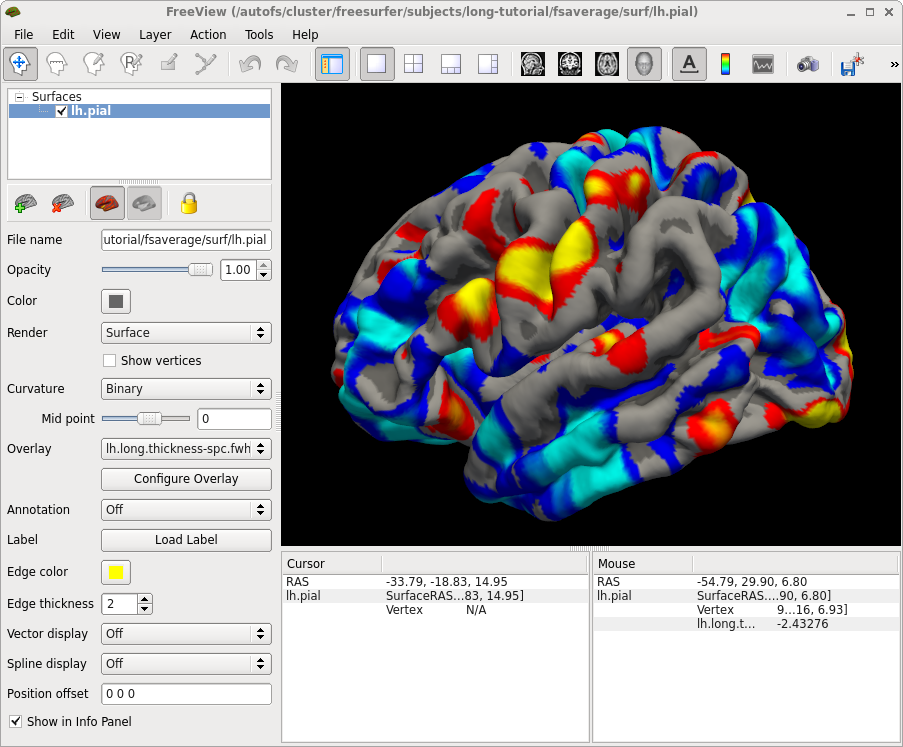
Click on the 3D view button if freeview opens in a different view from what is depicted in the screenshot below, then click somewhere on the cortex to see the time course data at that location.

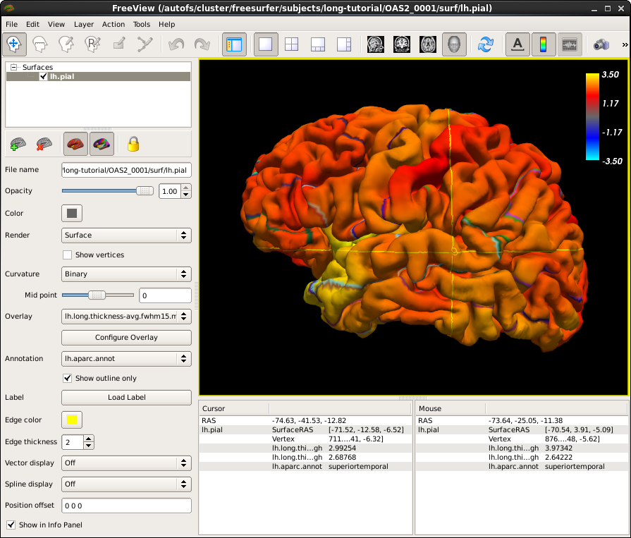
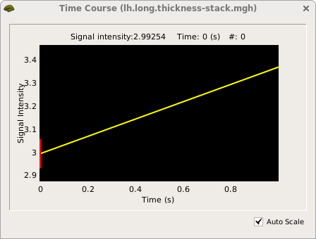
You are looking at the smoothed average thickness (color overlay) with values between 1 (red) and >3 mm (yellow). If you click at any location on the surface you can see a plot of the two original (unsmoothed) thickness values at the two time points. We also opened the cortical parcellation (aparc, using the annot flag) in outline style, which can be switched on and off. It helps to find out what region you are inspecting when clicking on the surface. For a single subject values are often noisy even after smoothing and show local thinning and thickening. That is why for a group analysis one needs several subjects in each group. The yellow lines/curves in the main window on the surface show the intersection of the three planes with the cortex at the selected location, and can be ignored.

For users with only an older Freeview version (no support for time course), you can use tksurfer to achieve the same (no need to do it in the course): tksurfer OAS2_0001 lh pial -overlay $SUBJECTS_DIR/OAS2_0001/surf/lh.long.thickness-avg.fwhm15.mgh -timecourse $SUBJECTS_DIR/OAS2_0001/surf/lh.long.thickness-stack.mgh -aparc

In a similar fashion you can open for example the symmetrized percent change. Close any open freeview windows. This time we open the overlay on fsaverage, an average subject provided with FreeSurfer and often used as the common target to compare results across subjects. The --qcache flag of long_mris_slopes has conveniently registered and mapped all results to this average subject:

freeview -f fsaverage/surf/lh.pial:overlay=$SUBJECTS_DIR/OAS2_0001/surf/lh.long.thickness-spc.fwhm15.fsaverage.mgh:overlay_threshold=2,5

note the 'fsaverage' in the filename. Because there is not much change on the surfaces, the SPC will be even more noisy than the average. You can use the above commands to investigate individual results, but this is rarely necessary.

Since FS5.2: Similar to the long_mris_slopes command above to compute thickness change, you can use long_stats_slopes to compute subject rates, percent changes, etc. for the ROI stats (aseg or aparc, i.e. subcortical and cortical ROI volumes and average thickness). Once you reduced the measures to a single number per subject, you can compare groups similar to a cross sectional analysis (e.g. using mri_glm_fit).

4.4. Additional Notes on QDEC

In order to run a QDEC group analysis (described in the QDEC tutorial), you need a qdec table. Since qdec cannot directly work with the longitudinal qdec tables yet, you have to shrink it into a cross sectional form. Use

long_qdec_table --qdec ./qdec/long.qdec.table.dat --cross --out ./qdec/cross.qdec.table.dat

to create a table with only a single line for each subject. For each subject, numerical values such as age or height will be averaged across time, other values will be copied from the first time point for each subject as ordered in the input table.

Also QDEC will not know about our new files (e.g. lh.long.thickness-spc...), that you created above with long_mris_slopes. We can tell it to look for them by creating a $SUBJECTS_DIR/qdec/.Qdecrc file (it needs to be in the qdec directory) that contains the following lines:

MEASURE1 = long.thickness-avg
MEASURE2 = long.thickness-rate
MEASURE3 = long.thickness-pc1
MEASURE4 = long.thickness-spc

(If you are running your own data, make sure you create this file in the $SUBJECTS_DIR/qdec directory!)

You can then run qdec and do all kinds of analysis on any of those files and other variables from the qdec table:

qdec --table ./qdec/cross.qdec.table.dat

You will see in the Design tab, that you can now select e.g. long.thickness-rate under Measure as the dependent variable. Check out the QDEC tutorial to see how to run a qdec analysis.

5. Editing Longitudinal Data

Editing longitudinal data can be complicated, but in some cases you actually save time, as some edits are only necessary in the base. You should be familiar with Edits and might want to check also the page about LongitudinalEdits.

Here are some examples of some common errors you can encounter with your data. Note: Because some of the recons take a while to run and it is not practical for you to run them during this short period of time, we ran the edits ahead of time. You will see that the edited and re-processed version have the postfix '_fixed'.

Before starting each section, remember to do the following to any new terminal you open:

export SUBJECTS_DIR=$TUTORIAL_DATA/long-tutorial
cd $SUBJECTS_DIR

5.0.1. Freeview Cheat Sheet

(You can skip this now and look at if later when editing, if you forgot how to use these tools)

Remember: in order to edit you must first click the Voxel editing box , then if you're editing the brainmask.mgz or wm.mgz You must click the "Recon Editing" box in the Voxel Edit window that pops up. It should look like this:

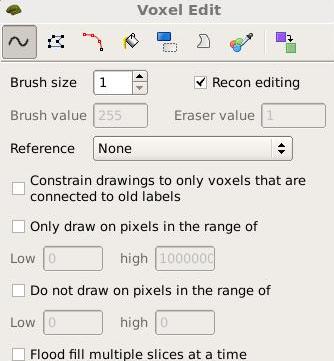
OR you can select this 'Recon Edit' button instead
If you're editing the aseg or any segmentation volume, you must uncheck this "Recon Editing" box in order to be able to erase voxels properly.

When editing in freeview, clicking with the left mouse button will draw voxels and holding down the shift key while clicking with the left mouse button will delete them. Make sure you're in "Recon Editing" mode when editing the wm.mgz or brainmask and that this box is unchecked when editing the aseg. Don't forget to save the volume you're working on when you're done by making sure the volume you want to save is highlighted and clicking or going to File --> Save Volume.
Control Points: To add control points, go to File --> New Point Set" name the file "control.dat, select the brainmask.mgz or T1.mgz as your template volume, and press OK. Clicking with your left mouse button will add a control point, holding down the shift key and clicking on an existing point will delete that control point. Don't forget to go to File --> Save Point Set or clicking when you're done and entering control.dat as the file name.
White Matter: To edit the wm.mgz, click on wm under the Volumes tab and set the "Color map" to "heat" so that you can see the brain underneath the wm.mgz. You can play with the opacity slider or use ALT-V to turn the wm.mgz on and off to aid in editing. Verify that you're in "Recon Editing" mode and use the left mouse key to add voxels and hold down the shift key and click to delete them. Don't forget to save the volume when you're done editing.

5.1. Skullstrip Error

The most common type of skull strip failures you probably will see has to do with the cerebellum: Often, part of the cerebellum is stripped off (as you have seen in the skull strip tutorial in the troubleshooting portion earlier). Sometimes skull stripping will also leave too much dura behind. For either case, the best way to solve the problem is to adjust the watershed parameters.

Very rarely, you will see FreeSurfer fail completely in the skullstrip step (usually associated with many other errors) as is clearly the case in the following example. For the purpose of this tutorial we will only focus on and fix the skull strip error in this case.

Please take a look at the base for subject OAS2_0004:

freeview -v OAS2_0004/mri/T1.mgz \
            OAS2_0004/mri/brainmask.mgz \
         -f OAS2_0004/surf/lh.pial:edgecolor=red \
            OAS2_0004/surf/rh.pial:edgecolor=red \
            OAS2_0004/surf/lh.white:edgecolor=blue \
            OAS2_0004/surf/rh.white:edgecolor=blue

This looks pretty bad. In order to find out what causes these problems it is important to also check the cross-sectional runs for the same subject to see if the problem is present there.

You can open the cross (in separate terminals, don't forget to set the SUBJECTS_DIR in a new terminal window):

freeview -v OAS2_0004_MR1/mri/T1.mgz \
            OAS2_0004_MR1/mri/brainmask.mgz \
         -f OAS2_0004_MR1/surf/lh.pial:edgecolor=red \
            OAS2_0004_MR1/surf/rh.pial:edgecolor=red \
            OAS2_0004_MR1/surf/lh.white:edgecolor=blue \
            OAS2_0004_MR1/surf/rh.white:edgecolor=blue

freeview -v OAS2_0004_MR2/mri/T1.mgz \
            OAS2_0004_MR2/mri/brainmask.mgz \
         -f OAS2_0004_MR2/surf/lh.pial:edgecolor=red \
            OAS2_0004_MR2/surf/rh.pial:edgecolor=red \
            OAS2_0004_MR2/surf/lh.white:edgecolor=blue \
            OAS2_0004_MR2/surf/rh.white:edgecolor=blue

Usually, if the base and cross runs were OK, you would also open the longs (in separate terminals), but that is not necessary here. For completeness, these would be the commands:

freeview -v OAS2_0004_MR1.long.OAS2_0004/mri/T1.mgz \
            OAS2_0004_MR1.long.OAS2_0004/mri/brainmask.mgz \
         -f OAS2_0004_MR1.long.OAS2_0004/surf/lh.pial:edgecolor=red \
            OAS2_0004_MR1.long.OAS2_0004/surf/rh.pial:edgecolor=red \
            OAS2_0004_MR1.long.OAS2_0004/surf/lh.white:edgecolor=blue \
            OAS2_0004_MR1.long.OAS2_0004/surf/rh.white:edgecolor=blue

freeview -v OAS2_0004_MR2.long.OAS2_0004/mri/T1.mgz \
            OAS2_0004_MR2.long.OAS2_0004/mri/brainmask.mgz \
         -f OAS2_0004_MR2.long.OAS2_0004/surf/lh.pial:edgecolor=red \
            OAS2_0004_MR2.long.OAS2_0004/surf/rh.pial:edgecolor=red \
            OAS2_0004_MR2.long.OAS2_0004/surf/lh.white:edgecolor=blue \
            OAS2_0004_MR2.long.OAS2_0004/surf/rh.white:edgecolor=blue

These commands will open the brainmask.mgz volume, the T1.mgz, and the surfaces for both hemispheres. You can check the brainmask.mgz volume and compare it to the T1.mgz volume (use Alt+v to toggle between them).

While looking at the base helps to see that this subject's processing has a problem, it is clear that the cross sectional processing already fails. You can see a description of how to fix it here along with the edited version.

5.2. Pial/Brainmask Edits

Sometimes you will come across a case where you need to make edits to the brainmask.mgz to correct the pial surfaces. Open subject OAS2_0057 to see where and how this type of edits should be done.

First open the base:

freeview -v OAS2_0057/mri/T1.mgz \
            OAS2_0057/mri/brainmask.mgz \
         -f OAS2_0057/surf/lh.pial:edgecolor=red \
            OAS2_0057/surf/rh.pial:edgecolor=red \
            OAS2_0057/surf/lh.white:edgecolor=blue \
            OAS2_0057/surf/rh.white:edgecolor=blue

This will open the brainmask.mgz volume, T1.mgz volume, and all surfaces. You should also check out the cross-sectionals and the longitudinals of this subject to check if the problem is present in all parts of the stream:

freeview -v OAS2_0057_MR1/mri/T1.mgz \
            OAS2_0057_MR1/mri/brainmask.mgz \
         -f OAS2_0057_MR1/surf/lh.pial:edgecolor=red \
            OAS2_0057_MR1/surf/rh.pial:edgecolor=red \
            OAS2_0057_MR1/surf/lh.white:edgecolor=blue \
            OAS2_0057_MR1/surf/rh.white:edgecolor=blue

freeview -v OAS2_0057_MR2/mri/T1.mgz \
            OAS2_0057_MR2/mri/brainmask.mgz \
         -f OAS2_0057_MR2/surf/lh.pial:edgecolor=red \
            OAS2_0057_MR2/surf/rh.pial:edgecolor=red \
            OAS2_0057_MR2/surf/lh.white:edgecolor=blue \
            OAS2_0057_MR2/surf/rh.white:edgecolor=blue

freeview -v OAS2_0057_MR1.long.OAS2_0057/mri/T1.mgz \
            OAS2_0057_MR1.long.OAS2_0057/mri/brainmask.mgz \
         -f OAS2_0057_MR1.long.OAS2_0057/surf/lh.pial:edgecolor=red \
            OAS2_0057_MR1.long.OAS2_0057/surf/rh.pial:edgecolor=red \
            OAS2_0057_MR1.long.OAS2_0057/surf/lh.white:edgecolor=blue \
            OAS2_0057_MR1.long.OAS2_0057/surf/rh.white:edgecolor=blue

freeview -v OAS2_0057_MR2.long.OAS2_0057/mri/T1.mgz \
            OAS2_0057_MR2.long.OAS2_0057/mri/brainmask.mgz \
         -f OAS2_0057_MR2.long.OAS2_0057/surf/lh.pial:edgecolor=red \
            OAS2_0057_MR2.long.OAS2_0057/surf/rh.pial:edgecolor=red \
            OAS2_0057_MR2.long.OAS2_0057/surf/lh.white:edgecolor=blue \
            OAS2_0057_MR2.long.OAS2_0057/surf/rh.white:edgecolor=blue

See if you can find the slices where you will need to edit the braimask.mgz in order to correct the surfaces. You can click here for a detailed description on how and at which stage you can fix this problem.

5.3. Control Points Edits

Sometimes, there are areas in the white matter with intensity lower than 110 and where the wm is not included in the surfaces. The best way to fix this problem is to add control points.

Take a look at the next subject, OAS2_0121 in all cross, base, and long to see if you can find the places that need control points.

freeview -v OAS2_0121_MR1/mri/T1.mgz \
            OAS2_0121_MR1/mri/brainmask.mgz \
         -f OAS2_0121_MR1/surf/lh.pial:edgecolor=red \
            OAS2_0121_MR1/surf/rh.pial:edgecolor=red \
            OAS2_0121_MR1/surf/lh.white:edgecolor=blue \
            OAS2_0121_MR1/surf/rh.white:edgecolor=blue

freeview -v OAS2_0121_MR2/mri/T1.mgz \
            OAS2_0121_MR2/mri/brainmask.mgz \
         -f OAS2_0121_MR2/surf/lh.pial:edgecolor=red \
            OAS2_0121_MR2/surf/rh.pial:edgecolor=red \
            OAS2_0121_MR2/surf/lh.white:edgecolor=blue \
            OAS2_0121_MR2/surf/rh.white:edgecolor=blue

freeview -v OAS2_0121/mri/T1.mgz \
            OAS2_0121/mri/brainmask.mgz \
         -f OAS2_0121/surf/lh.pial:edgecolor=red \
            OAS2_0121/surf/rh.pial:edgecolor=red \
            OAS2_0121/surf/lh.white:edgecolor=blue \
            OAS2_0121/surf/rh.white:edgecolor=blue

freeview -v OAS2_0121_MR1.long.OAS2_0121/mri/T1.mgz \
            OAS2_0121_MR1.long.OAS2_0121/mri/brainmask.mgz \
         -f OAS2_0121_MR1.long.OAS2_0121/surf/lh.pial:edgecolor=red \
            OAS2_0121_MR1.long.OAS2_0121/surf/rh.pial:edgecolor=red \
            OAS2_0121_MR1.long.OAS2_0121/surf/lh.white:edgecolor=blue \
            OAS2_0121_MR1.long.OAS2_0121/surf/rh.white:edgecolor=blue

freeview -v OAS2_0121_MR2.long.OAS2_0121/mri/T1.mgz \
            OAS2_0121_MR2.long.OAS2_0121/mri/brainmask.mgz \
         -f OAS2_0121_MR2.long.OAS2_0121/surf/lh.pial:edgecolor=red \
            OAS2_0121_MR2.long.OAS2_0121/surf/rh.pial:edgecolor=red \
            OAS2_0121_MR2.long.OAS2_0121/surf/lh.white:edgecolor=blue \
            OAS2_0121_MR2.long.OAS2_0121/surf/rh.white:edgecolor=blue

Click here if you want to see where to place the control points and what effects it has on the longitudinals.

5.4. White Matter Edits

White matter edits are possibly the most common type of edits you will come across in data. In many cases, even a difference of 1 wm voxel can cause a huge defect in the surfaces. Take a look at the following subject. For this one, we will open the brainmask.mgz volume and the wm.mgz volume as aux instead of T1.mgz.

freeview -v OAS2_0185/mri/wm.mgz \
            OAS2_0185/mri/brainmask.mgz \
         -f OAS2_0185/surf/lh.pial:edgecolor=red \
            OAS2_0185/surf/rh.pial:edgecolor=red \
            OAS2_0185/surf/lh.white:edgecolor=blue \
            OAS2_0185/surf/rh.white:edgecolor=blue

freeview -v OAS2_0185_MR1/mri/wm.mgz \
            OAS2_0185_MR1/mri/brainmask.mgz \
         -f OAS2_0185_MR1/surf/lh.pial:edgecolor=red \
            OAS2_0185_MR1/surf/rh.pial:edgecolor=red \
            OAS2_0185_MR1/surf/lh.white:edgecolor=blue \
            OAS2_0185_MR1/surf/rh.white:edgecolor=blue

freeview -v OAS2_0185_MR2/mri/wm.mgz \
            OAS2_0185_MR2/mri/brainmask.mgz \
         -f OAS2_0185_MR2/surf/lh.pial:edgecolor=red \
            OAS2_0185_MR2/surf/rh.pial:edgecolor=red \
            OAS2_0185_MR2/surf/lh.white:edgecolor=blue \
            OAS2_0185_MR2/surf/rh.white:edgecolor=blue

freeview -v OAS2_0185_MR1.long.OAS2_0185/mri/wm.mgz \
            OAS2_0185_MR1.long.OAS2_0185/mri/brainmask.mgz \
         -f OAS2_0185_MR1.long.OAS2_0185/surf/lh.pial:edgecolor=red \
            OAS2_0185_MR1.long.OAS2_0185/surf/rh.pial:edgecolor=red \
            OAS2_0185_MR1.long.OAS2_0185/surf/lh.white:edgecolor=blue \
            OAS2_0185_MR1.long.OAS2_0185/surf/rh.white:edgecolor=blue

freeview -v OAS2_0185_MR2.long.OAS2_0185/mri/wm.mgz \
            OAS2_0185_MR2.long.OAS2_0185/mri/brainmask.mgz \
         -f OAS2_0185_MR2.long.OAS2_0185/surf/lh.pial:edgecolor=red \
            OAS2_0185_MR2.long.OAS2_0185/surf/rh.pial:edgecolor=red \
            OAS2_0185_MR2.long.OAS2_0185/surf/lh.white:edgecolor=blue \
            OAS2_0185_MR2.long.OAS2_0185/surf/rh.white:edgecolor=blue

Toggle between the two volumes (use the opacity slider) and see if you can spot an area where a simple wm edit will make a huge difference to the surfaces. Once you find it, or if you give up, click here to see how the edits can be done.

5.5. Brain.finalsurfs.manedit.mgz Edits

The brain.finalsurfs.manedit.mgz volume will allow for the correction of a particular type of problem involving pial surface misplacement whereby parts of the pial surface have extended into the cerebellum in certain areas. It is only in this case where the pial surface extends into cerebellum where the brain.finalsurfs.manedit.mgz volume should be edited. In all other non-cerebellum pial surface problems, brainmask.mgz should be edited. This cerebellum/pial surface problem can be fixed by removing those cerebellum voxels and other surrounding problematic voxels in the brain.finalsurfs.manedit.mgz volume such that upon running recon-all, the pial surface will be pulled in as desired, bordering only gray matter/ CSF boundary, and not jutting into the cerebellum. If only edits to this volume are made on a subject, it is sufficient to re-run recon-all from the point of these edits using the flag -autorecon3-pial. For the following subject (OAS2_0002), it is seen that both cross sectional time points (OAS2_0002_MR1 and OAS2_0002_MR2) have some errors of this nature in several slices of the brain.finalsurfs.mgz volume. In the corresponding region in the base (OAS2_0002), similar problems show up, and therefore, the longitudinal data sets for time points 1 and 2 also have some errors in the corresponding areas of the brain.finalsurfs.mgz volume. The tutorial below demonstrates how to manually fix the problem in the cross sectional time points and in the base, in order to automatically fix the problem in the long. Notice that edits will be made to a copy of the brain.finalsurfs.mgz file which will be named brain.finalsurfs.manedit.mgz. The tutorial walks you through editing cross-sectional time point 2 step by step, because the error in question is larger and better defined in this time point as compared to time point 1. However, the tutorial explains how to fix the problem in time point 1 as well. In practice, you should check both cross-sectional time points for errors of this type, fix them and regenerate the crosssectionals. Then, you should check the base, fix any errors, and regenerate the base. Then, regenerate both longitudinal runs using the fixed cross-sectional data sets and the fixed base.

1. Look at the brain.finalsurfs.mgz volumes within OAS2_0002_MR2 at the slices containing cerebellum in order to see the problem.

freeview -v OAS2_0002_MR2/mri/brain.finalsurfs.mgz \
            OAS2_0002_MR2/mri/aseg.mgz:colormap=lut:opacity=0.25 \
         -f OAS2_0002_MR2/surf/lh.pial:edgecolor=red \
            OAS2_0002_MR2/surf/rh.pial:edgecolor=red \
            OAS2_0002_MR2/surf/lh.white:edgecolor=blue \
            OAS2_0002_MR2/surf/rh.white:edgecolor=blue

Click here to view the problem and how to fix it.

Reminder: once you start making edits to the brain.finalsurfs.mgz save as brain.finalsurfs.manedit.mgz!

2. Editing the Base: Open the base for this subject

freeview -v OAS2_0002/mri/brain.finalsurfs.mgz \
            OAS2_0002/mri/aseg.mgz:colormap=lut:opacity=0.25 \
         -f OAS2_0002/surf/lh.pial:edgecolor=red \
            OAS2_0002/surf/rh.pial:edgecolor=red \
            OAS2_0002/surf/lh.white:edgecolor=blue \
            OAS2_0002/surf/rh.white:edgecolor=blue

Click here to view the problem and how to fix it.

Reminder: once you start making edits to the brain.finalsurfs.mgz save as brain.finalsurfs.manedit.mgz!

3. Once the cross-sectional time points 1 and 2 and the base are fixed, it is time to recreate a long files for time points 1 and 2 (by renaming/removing the old and re-processing the -long from scratch). First you can view the original long data for time point 2 (for example) below:

freeview -v OAS2_0002_MR2.long.OAS2_0002/mri/brain.finalsurfs.mgz \
            OAS2_0002_MR2.long.OAS2_0002/mri/aseg.mgz:colormap=lut:opacity=0.25 \
         -f OAS2_0002_MR2.long.OAS2_0002/surf/lh.pial:edgecolor=red \
            OAS2_0002_MR2.long.OAS2_0002/surf/rh.pial:edgecolor=red \
            OAS2_0002_MR2.long.OAS2_0002/surf/lh.white:edgecolor=blue \
            OAS2_0002_MR2.long.OAS2_0002/surf/rh.white:edgecolor=blue

Click here to see the results of creating a new long file from the edited base and cross-sectional. You will do the same for MR1.

Reminder: once you start making edits to the brain.finalsurfs.mgz save as brain.finalsurfs.manedit.mgz!

MartinReuter