• FsFastTutorialV5.1
• FsFastFirstLevel_freeview

top | previous (Preprocessing)| Next (Group Analysis)

1. First Level (Time Series) Analysis

This tutorial describes how to analyze the time series data by configuring analyses (design matrices) and contrasts. There are two distinct stages:

1. Configuring analyses and contrasts
2. Analyzing the data by fitting the time courses to the model and computing p-values for contrasts

Start the tutorial in the Project directory:

export SUBJECTS_DIR=$TUTORIAL_DATA/fsfast-tutorial.subjects
cd $TUTORIAL_DATA/fsfast-functional

2. Configure an Analysis

The first step in the first-level analysis is to configure analyses and contrasts. This step describes what preprocessing stages should have been run as well as the parameters needed to construct a design matrix (no data are analyzed yet). This is done with mkanalysis-sess

mkanalysis-sess \
  -fsd bold -stc up  -surface fsaverage lh -fwhm 5  \
  -event-related  -paradigm workmem.par -nconditions 5 \
  -spmhrf 0 -TR 2 -refeventdur 16 -nskip 4 -polyfit 2 \
  -analysis my-workmem.sm05.lh -force -per-run

• -fsd bold -stc up -surface fsaverage lh -fwhm 5 : preprocessing options (see preproc-sess). There needs to be a separate analysis configuration for each space (ie, lh, rh, mni305)

• -event-related : for event-related and blocked designs

• -paradigm workmem.par : name of paradigm file

• -nconditions 5 : number of conditions to expect in paradigm file
• -spmhrf 0 : use canonical SPM HRF with 0 derivatives
• -TR 2 : expect raw data to have a 2 sec TR
• -refeventdur 16 : scale amplitudes based on a 16 sec event duration
• -nskip 4 : skip the first four time points (paradigm timing still ok)
• -polyfit 2 : use 2nd order polynomial nuisance regressors
• -analysis my-workmem.sm05.lh : this is the name of the analysis configuration. Choose a descriptive name (and one that includes the space)
• -force : overwrite any existing analysis

To construct the design matrix there are several pieces of information that are given in the above command:

• The stimulus timing (obtained from a file called workmem.par in the Run directory)
• The hemodynamic response model (SPM canonical shape (-spmhrf))
• Nuisance regressors: 2nd order polynomial (-polyfit 2) and skipping first 4 time points (-nskip 4)

This command finishes within seconds. It creates a folder called my-workmem.sm05.lh. See the contents with

ls my-workmem.sm05.lh

There will be a text file called 'analysis.info' with a list of all the parameters that you just specified. There is enough information here that the raw data and paradigm files can be found and the entire design matrix constructed. No data have been analyzed yet!

3. Configure Contrasts

Contrasts are embodiments of hypotheses that you want to test. They are linear combinations of conditions. In order to construct a contrast, you need to know the numeric ID associated with each condition; this is specified in the workmem.par paradigm file. For this design, the conditions are

1. Encode
2. Emotional Distractor
3. Neutral Distractor
4. Probe After Emotional Distractor
5. Probe After Neutral Distractor

In a contrast, a weight must be assigned to each each condition. Often, the weights are 0, +1, or -1.

3.1. Encode vs Baseline Contrast

To find voxels that are activated by the Encode condition relative to baseline, one would assign a weight of 1 to Encode and 0 to everything else (ie, the contrast vector would be [1 0 0 0 0]). There is a value for each of the 5 conditions. The first value (for Encode) is 1, the rest are 0. To create this contrast matrix in FSFAST, run

mkcontrast-sess -analysis my-workmem.sm05.lh -contrast encode-v-base -a 1

• -analysis my-workmem.sm05.lh : analysis name from mkanalysis-sess above
• -contrast encode-v-base : name of the contrast. Choose something descriptive
• -a 1 : set the weight for condition 1 to be +1 (-a means 'active')
• By default, all other conditions given a weight of 0

This will finish in a few seconds (still no data have been analyzed!), creating a files called 'encode-v-base.mat' in my-workmem.sm05.lh

ls my-workmem.sm05.lh

This is a binary matlab file and cannot be viewed.

3.2. Emotional Distractor vs Neutral Distractor

The Emotional Distractor is the second condition, and the Neutral Distractor is the third condition. To find voxels that are activated by Emotional more than Neutral, one would need the following contrast vector [0 1 -1 0 0]. This is achieved with the command:

mkcontrast-sess -analysis my-workmem.sm05.lh -contrast emot.dist-v-neut.dist -a 2 -c 3

• -contrast emot.dist-v-neut.dist : name of the contrast.
• -a 2 : set the weight for condition 2 to be +1 (-a means 'active')
• -c 3 : set the weight for condition 3 to be -1 (-c means 'control')
• All other conditions given a weight of 0
• Creates emot.dist-v-neut.dist.mat in my-workmem.sm05.lh

3.3. Distractor Average vs Baseline

One may be interested in voxels that respond to either Emotional or Neutral Distractor. This can be achieved by testing the average of the two distractors against baseline. One would need the following contrast vector [0 0.5 0.5 0 0]. When there are multiple '-a' conditions, FSFAST automatically rescales the weights so that the positives sum to 1 (mutiple '-c' conditions will sum to -1). This is achieved with the command:

mkcontrast-sess -analysis my-workmem.sm05.lh -contrast distractor.avg-v-base -a 2 -a 3

• -contrast distractor.avg-v-base : name of the contrast.
• -a 2 : set the weight for condition 2 to be +1 (-a means 'active')
• -a 3 : set the weight for condition 3 to be +1 (-a means 'active')
• All other conditions given a weight of 0
• Creates distractor.avg-v-base.mat in my-workmem.sm05.lh

3.4. Emotional Distractor vs Baseline Contrast

The Emotional Distractor is the second condition, so, to find voxels that are activated by it relative to baseline, one would need the following contrast vector [0 1 0 0 0]. This is achieved with the command:

mkcontrast-sess -analysis my-workmem.sm05.lh -contrast emot.dist-v-base -a 2

• -contrast emot.dist-v-base : name of the contrast. Choose something descriptive
• -a 2 : set the weight for condition 2 to be +1 (-a means 'active')
• By default, all other conditions given a weight of 0
• Creates emot.dist-v-base.mat in my-workmem.sm05.lh

3.5. Probe Average vs Baseline

The Probes are conditions 4 and 5. If we are interested in the voxels activated by a probe regardless of whether it follows an emotional or neutral distractor, then we can create a contrast in which we average their amplitudes: [0 0 0 0.5 0.5]. This is achieved with the command:

mkcontrast-sess -analysis my-workmem.sm05.lh -contrast probe.avg-v-base -a 4 -a 5

• -contrast probe.avg-v-base : name of the contrast.
• -a 4 : set the weight for condition 4 to be +1
• -a 5 : set the weight for condition 5 to be +1
• All other conditions given a weight of 0

When more than one active condition are specified, the weights are rescaled so that they sum to 1, so the weights for conditions 4 and 5 will be 0.5 instead of 1. If more than one control are given, the weights are scaled so that they sum to -1.

4. Configurations for Other Spaces

The commands above will configure the analysis and contrast only for raw data sampled to the left hemisphere of fsaverage. To do a full brain analysis, you will need to configure analyses for the right hemisphere and for the mni305 (for subcortical): For the right hemisphere, use the same command as above with 'lh' changed to 'rh' in the '-surface' option and in the analysis name.

mkanalysis-sess \
  -fsd bold -stc up  -surface fsaverage rh -fwhm 5  \
  -event-related  -paradigm workmem.par -nconditions 5 \
  -spmhrf 0 -TR 2 -refeventdur 16 -nskip 4 -polyfit 2 \
  -analysis my-workmem.sm05.rh -force -per-run

You would need to create contrasts for rh as above (but do not need to to finish the tutorial).

For mni305, use the same command as above replacing '-surface fsaverage lh' with '-mni305 2'. The '2' indicates 2mm sampling. The name is changed to reflect mni305:

mkanalysis-sess \
  -fsd bold -stc up  -mni305 2 -fwhm 5  \
  -event-related  -paradigm workmem.par -nconditions 5 \
  -spmhrf 0 -TR 2 -refeventdur 16 -nskip 4 -polyfit 2 \
  -analysis my-workmem.sm05.mni305 -force -per-run

You would need to create contrasts for mni305 as above (but do not need to to finish the tutorial). Note. This does not need to be repeated for each sessid.

5. Summary of Analysis and Contrast Configurations

• Configure analyses and contrasts once regardless of number of subjects
• Configure an analysis and contrasts separately for lh, rh, and mni305
• Configurations only create files and folder in Project Directory
• Actual analysis done separately

6. First Level Analysis

The First Level analysis is the process of fitting the time series data to the model specified with mkanalysis-sess above) as well as computing contrasts. The command to do this in FSFAST is:

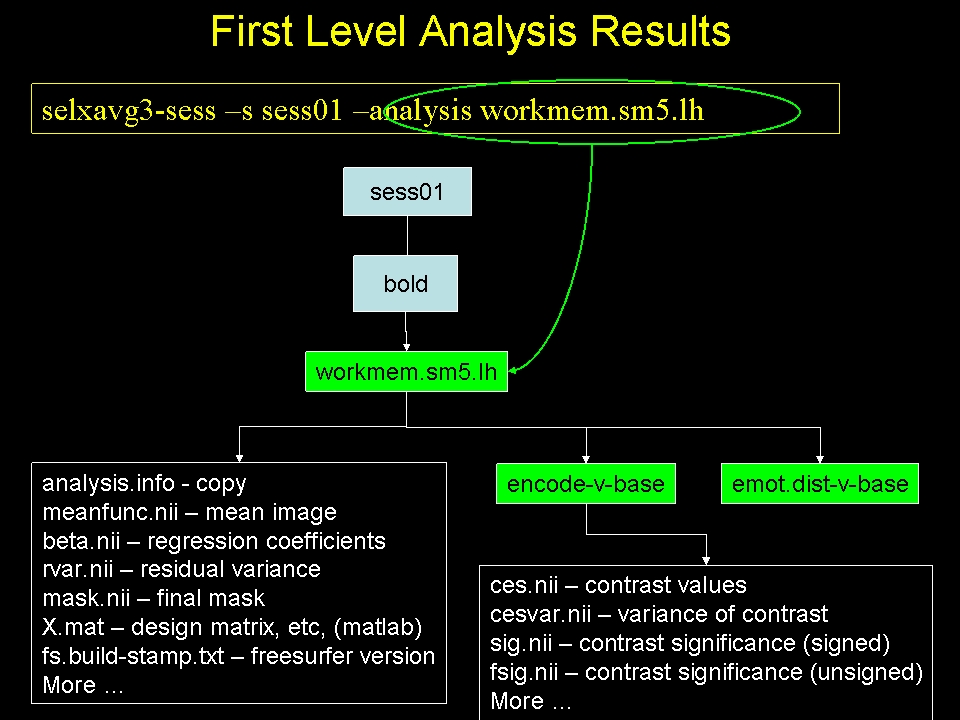
selxavg3-sess -s sess01 -analysis workmem.sm05.lh

• -s sess01 : session to analyze (can use -sf SessIdFile)

• -analysis workmem.sm05.lh : analysis configuration [Note: changed from my-workmem.sm05.lh]
• May take minutes or hours to complete

selxavg3-sess will:

• Automatically find preprocessed data and paradigm files
• Construct design matrix
• Construct contrast matrices
• Combine all Runs found in the FSD
• Compute regression coefficients (betas)
• Compute contrasts ane their significances
• Must run for each configuration (ie, workmem.sm05.{lh,rh,mni305})

This creates a new directory in the FSD for this session:

ls $TUTORIAL_DATA/fsfast-functional/sess01/bold

You will see 'workmem.sm05.lh' (as well as 'workmem.sm05.rh' and 'workmem.sm05.mni305'). For the most part, it is not necessary to know what the actual contents of the output are, but knowing about the output can help to demystify the process.

6.1. Visualize the First Level Output

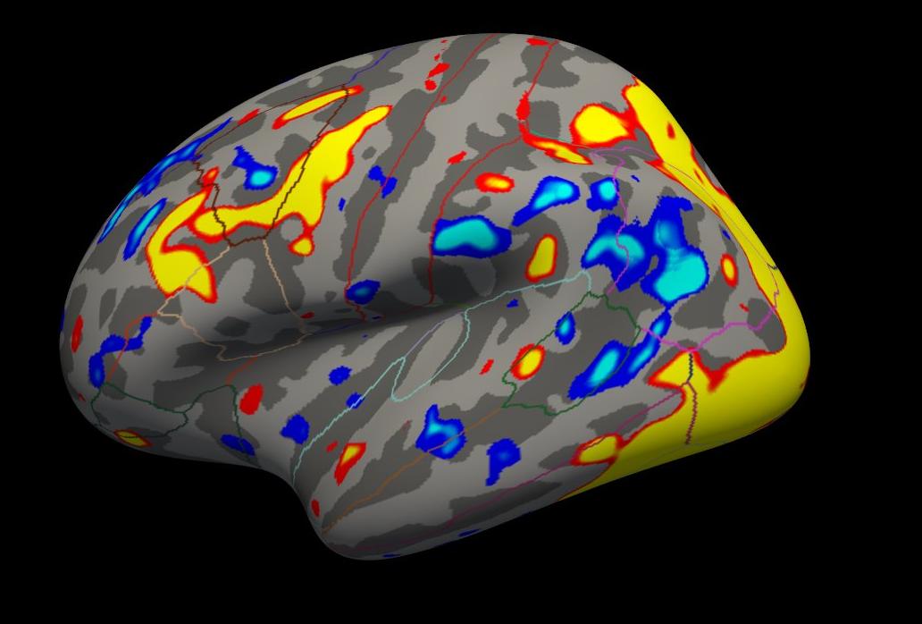
Bring up freeview to to look at the contrasts for the analysis in the fsaverage left hemisphere space:

tksurfer-sess -s sess01 \
  -analysis workmem.sm05.lh \
  -c encode-v-base \
  -c emot.dist-v-base \
  -c probe.avg-v-base \
  -c emot.dist-v-neut.dist \
  -freeview

• -s sess01 : session to view (cannot use -sf in this case)
• -analysis workmem.sm05.lh : analysis to view
• -c encode-v-base ... : load four contrasts in the given order

• Shows 'signifiances', ie, -log10(p). So, for p=.01, sig=2.

• Red/Yellow are for positive contrasts (eg, Enocode > Baseline)

• Blue/Cyan are for negative contrasts (eg, Enocode < Baseline)

To view the different contrasts:

• Click "Configure Overlay" in the sidebar.
• The "Frame" box will go from 0 to 3 corresponding to the four contrasts in the order entered on the command line.
• Adjust the "Frame" number or slider to see the different contrasts.
• You will need to reduce the threshold to see activation in the Emotional vs Neutral Distractor contrast.

To view the right hemisphere, use the same command as above, just change 'lh' to 'rh' (note: the right hemisphere is analyzed with a separate selxavg3-sess command).

tksurfer-sess -s sess01 \
  -analysis workmem.sm05.rh \
  -c encode-v-base \
  -c emot.dist-v-base \
  -c emot.dist-v-neut.dist \
  -c probe.avg-v-base \
  -freeview

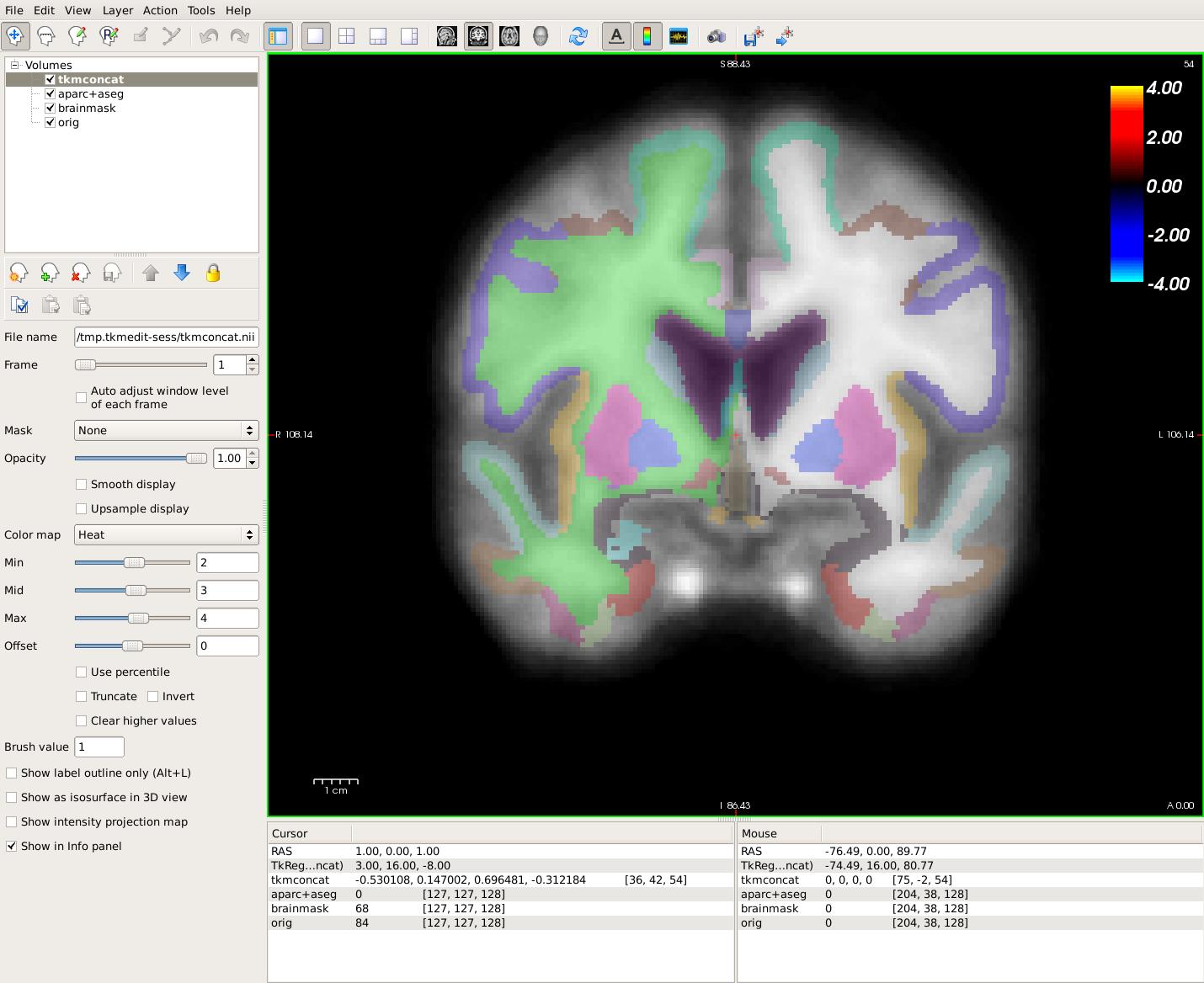
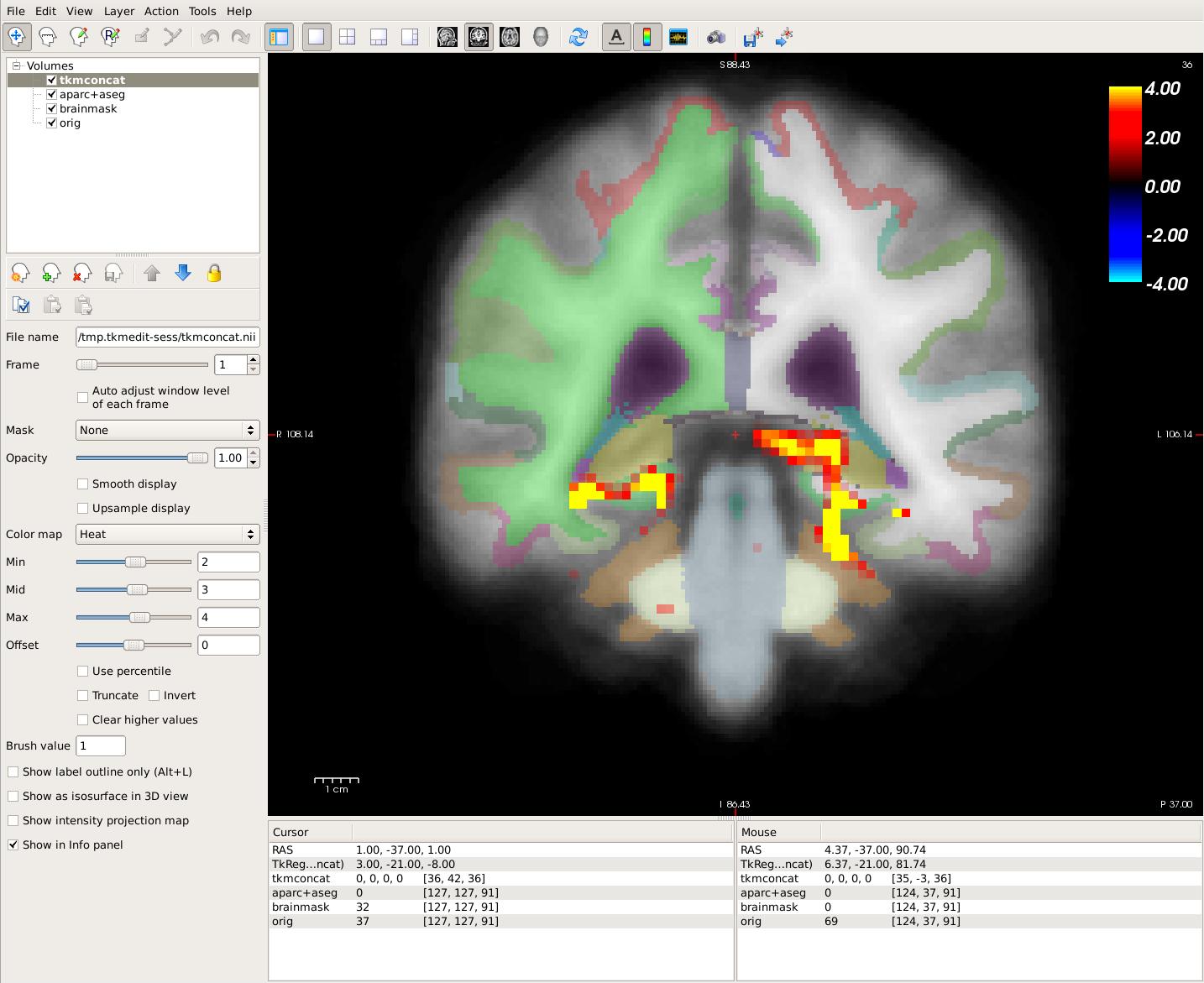
To view the volume-based analysis, the tool is freeview, and the rest of the command line is similar (just replace 'lh' with 'mni305'). (note: the mni305 is analyzed with a separate selxavg3-sess command).

tkmedit-sess -s sess01 -analysis workmem.sm05.mni305 \
  -c encode-v-base \
  -c emot.dist-v-base \
  -c emot.dist-v-neut.dist \
  -c probe.avg-v-base \
  -freeview

• top image (coronoal slice 128)
• bottom image: hippocampal activation (coronoal slice 91)
• These images show both cortical and subcortical areas.
• There is no activation in cortex because it has been masked out since it is analysed in cortical stream.

6.2. First-Level Analysis Summary

• Configure Analysis and contrasts once regardless of number of sessions
• Run selxavg3-sess for each space (lh, rh, mni305) for each session
• selxavg3-sess creates design matrix, fits parameters, computes contrasts and significances.
• Visualize surface-based analysis results with tksurfer-sess
• Visualize volume

7. Study Questions

• Configure a contrast for Probe following Emotional Distractor vs Probe following Neutral Distractor. Answer.

• How would you configure an analysis with a paradigm file called wmfir.par? Answer.

• How many times will you need to run mkanalysis-sess? Answer.

• How many times will you need to run selxavg3-sess? Answer.

8. First Level Output Details (Skip or Defer for FreeSurfer Course)

For the most part, it is not necessary to know what the actual contents of the output are, but knowing about the output can help to demystify the process. The output is going to go into the FSD of the given session.

cd sess01/bold
ls

You will see a folder called 'workmem.sm05.lh'. This is the output directory. View the contents of this directory:

cd workmem.sm05.lh
ls

There will be many files and folders. Some of the important ones are:

• analysis.info - copy from analysis configuration
• mask.nii.gz - mask combined from all individual runs
• beta.nii.gz - map of regression coefficients
• rvar.nii.gz - map of residual variances
• fsnr.nii.gz - map of the functional SNR
• encode-v-base - contrast folder
• emot.dist-v-base - contrast folder
• emot.dist-v-neut.dist - contrast folder
• probe.avg-v-base - contrast folder

Check the dimensions of mask.nii.gz with mri_info to verify that they are '163842 1 1 1', indicating that this is a surface with one frame (the mask). All 'volumes' in this folder will be this size. Go into one of the contrast directories:

cd encode-v-base
ls

Again, there are many files here. Some of the more important ones are:

• sig.nii.gz - voxel-wise significances as visualized above.
• ces.nii.gz - contrast values (like CON in SPM or COPE in FSL)
• cesvar.nii.gz - variance of contrast values (like VARCOPE in FSL)
• cespct.nii.gz - contrast values, percent computed on a voxel-wise basis
• cesvarpct.nii.gz - variance of percent contrast values
• t.nii.gz - t-ratio used to compute the sig.nii.gz
• pcc.nii.gz - partial correlation coefficient
• The ces and cesvar files are passed up to the higher level analysis.

top | previous (Preprocessing)| Next (Group Analysis)