• FsFastTutorialV6.0
• FsFastGroupLevelPerm

Back to list of all tutorials | Back to course page | FS-FAST Tutorial Homepage | Previous (First Level Analysis)

***NOTE: This group analysis tutorial uses permutation to correct for multiple comparisons. The cluster-wise p-values will be more accurate with permutation than with Monte Carlo simulation and GRF (our previous method). In general, the Monte Carlo p-values are too liberal (ie, they are more likely to imply that an effect is there when it really is not). The disadvantage to permutation is that it requires more processing time. Monte Carlo and GRF are NOT suitable for fMRI group analysis unless you use a rigorous threshold (e.g, a threshold of 3 (p<.001)), but it is important to note that at such high thresholds, you often don't see any significant voxels anyway.

If you are looking for the older version of this tutorial that uses Monte Carlo and GRF, click here.

1. Group Level Analysis

In general, the group analysis for fMRI is very similar to that of the structural data. There is a tutorial for this at GroupAnalysis. There are several specific differences for fMRI which are described here. In the structural Group Analysis, you would:

1. Run mris_preproc to resample each subject into the common space and then concatenate all of your subjects (one subject for each frame) into one file.
2. Smooth the data on the surface, then
3. Run mri_glmfit and mri_glmfit-sim

For the functional MRI group analysis you will need to:

1. Perform the following in each space (lh, rh, and mni305):
   • Concatenate individuals into one file (isxconcat-sess)
   • Do not smooth (already smoothed during first-level analysis)
   • Run mri_glmfit
   • Correct for multiple comparisons
2. Then:
   • Correct for multiple comparisons across the three spaces
   • Optionally merge the three spaces into one volume space

Start the tutorial in the Project directory

export SUBJECTS_DIR=$TUTORIAL_DATA/fsfast-tutorial.subjects
cd $TUTORIAL_DATA/fsfast-functional

2. Concatenating the Data

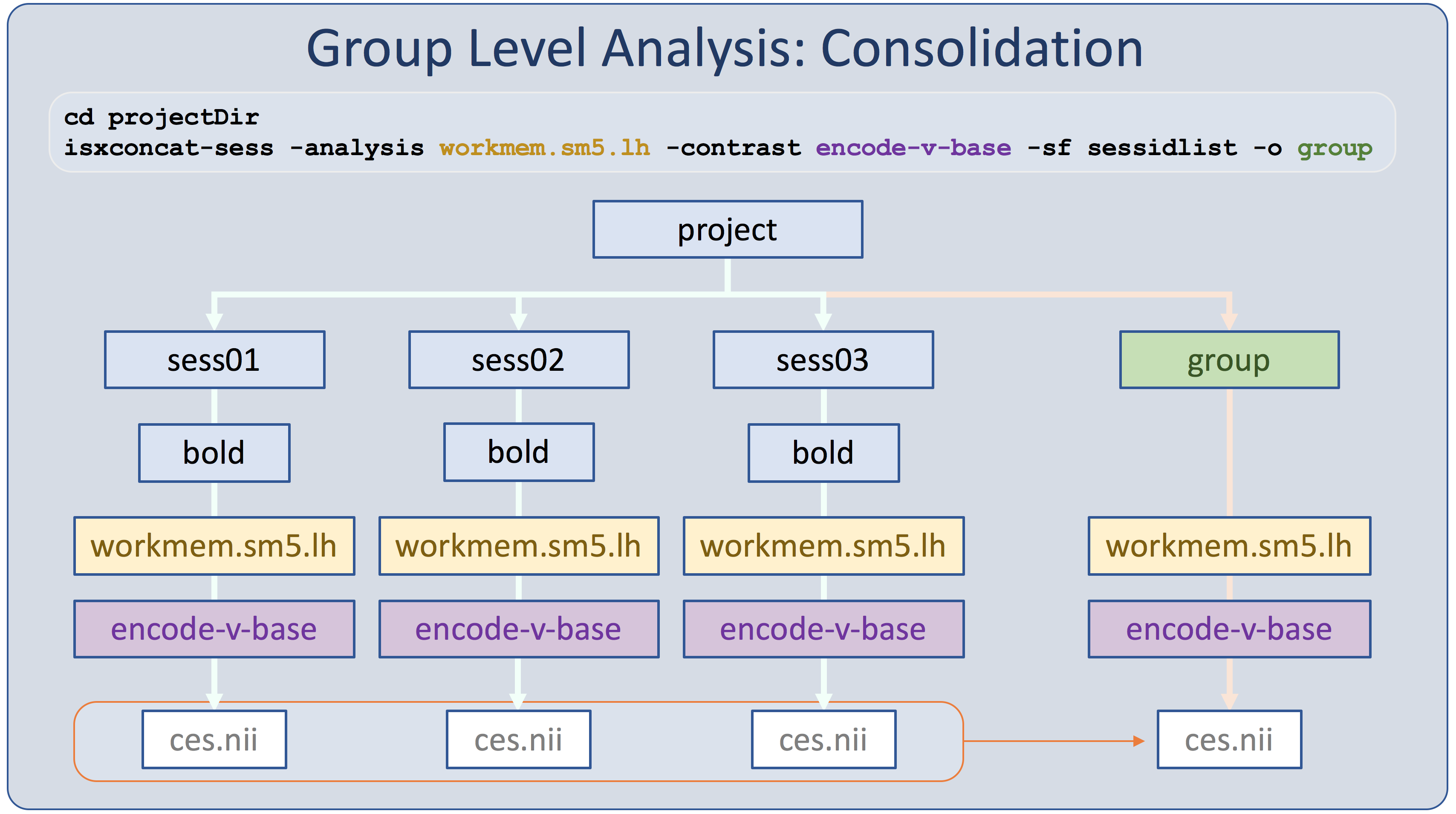
In the structural stream (see GroupAnalysis), the subjects' data were concatenated into one file with mris_preproc. For the functional stream, the program is called isxconcat-sess:

isxconcat-sess -sf sessidlist -analysis workmem.sm05.lh -contrast encode-v-base -o group

• -sf sessidlist : use all the subjects listed in sessidlist (order is important!)
• -analysis workmem.sm05.lh : analysis from mkanalysis-sess and selxavg3-sess
• -contrast encode-v-base : contrast from mkcontrast-sess. You can specify multiple contrasts with multiple -contrast flags.
• -o group : output folder is called 'group'
• Note: -all-contrasts can be used instead of -contrast.
  • Gets the contrast values (ces.nii.gz) for each subject and concatenates them into one file
  • Does the same for the contrast variances (cesvar.nii.gz)
  • Creates other files as well that can be used for checking for quality

"Isxconcat-sess" stands for "intersubject concatentation." This is a more recent version of the program, designed to work with selxavg3-sess. The x was added to keep versions consistent.

Run the concatenation for the right hemisphere and mni305 spaces:

isxconcat-sess -sf sessidlist -analysis workmem.sm05.rh -contrast encode-v-base -o group
isxconcat-sess -sf sessidlist -analysis workmem.sm05.mni305 -contrast encode-v-base -o group

When this is complete, cd into the 'group' directory and see what was created (this directory will also contain other sample data, ignore this for now)

cd $TUTORIAL_DATA/fsfast-functional/group
ls

• grouplist.txt : list of the sessions

• subjectlist.txt : list of the corresponding FreeSurfer subject IDs

• workmem.sm05.lh - left hemisphere analysis output folder
• workmem.sm05.rh - right hemisphere analysis output folder
• workmem.sm05.mni305 - MNI 305 analysis output folder

Go into the workmem.sm05.lh and see what's there:

cd $TUTORIAL_DATA/fsfast-functional/group/workmem.sm05.lh
ls

You will see several files and folders:

• analysis.info - copy of the analysis.info created by mkanalysis-sess
• meanfunc.nii.gz - a stack of the mean functional images for each session
• masks.nii.gz - a stack of the masks of all the individual subjects
• mask.nii.gz - a single mask based on the intersection of all masks
• fsnr.nii.gz - a stack of the functional SNRs for each session
• ffxdof.dat - text file with the total number of DOF summed over all sessions
• encode-v-base - folder with lower-level contrasts for the group of sessions

Each of the volumes are in the output space (lh, rh, mni305), as can be verified with mri_info. Go into the contrast folder and see what's there:

cd $TUTORIAL_DATA/fsfast-functional/group/workmem.sm05.lh/encode-v-base
ls

• ces.nii.gz - stack of all the contrast values from the lower level, one for each session
• cesvar.nii.gz - stack of all the contrast variances from the lower level, one for each session

These are going to be the inputs for the group GLM analysis.

3. Run the Group GLM for the Left Hemisphere

Details on how to run the GLM are given in Group Analysis, including the use of FSGD files to construct complicated group-level design matrices. Here we are going to use a very simple design which tests whether the mean across the groups equals 0 (the One Sample Group Mean, or OSGM). This just requires a design matrix with a single column of all ones (created with the --osgm flag):

mri_glmfit --y ces.nii.gz \
  --osgm \
  --surface fsaverage lh \
  --glmdir my-glm\
  --save-eres \
  --nii.gz

• --y ces.nii.gz : the input values to analyze
• --osgm : use One-Sample Group Mean
• --surface fsaverage lh : indicates surface-based data (not used for volume data)
• --glmdir my-glm : output directory
• --save-eres : save residual error (needed with permutation)
• --nii.gz : use compressed NIFTI as output format
• Note --wls is no longer recommended because it is incompatible with permutation

3.1. Visualize the Results of the Group GLM

tksurferfv fsaverage lh inflated -aparc -overlay my-glm/osgm/sig.nii.gz -fminmax 2 3

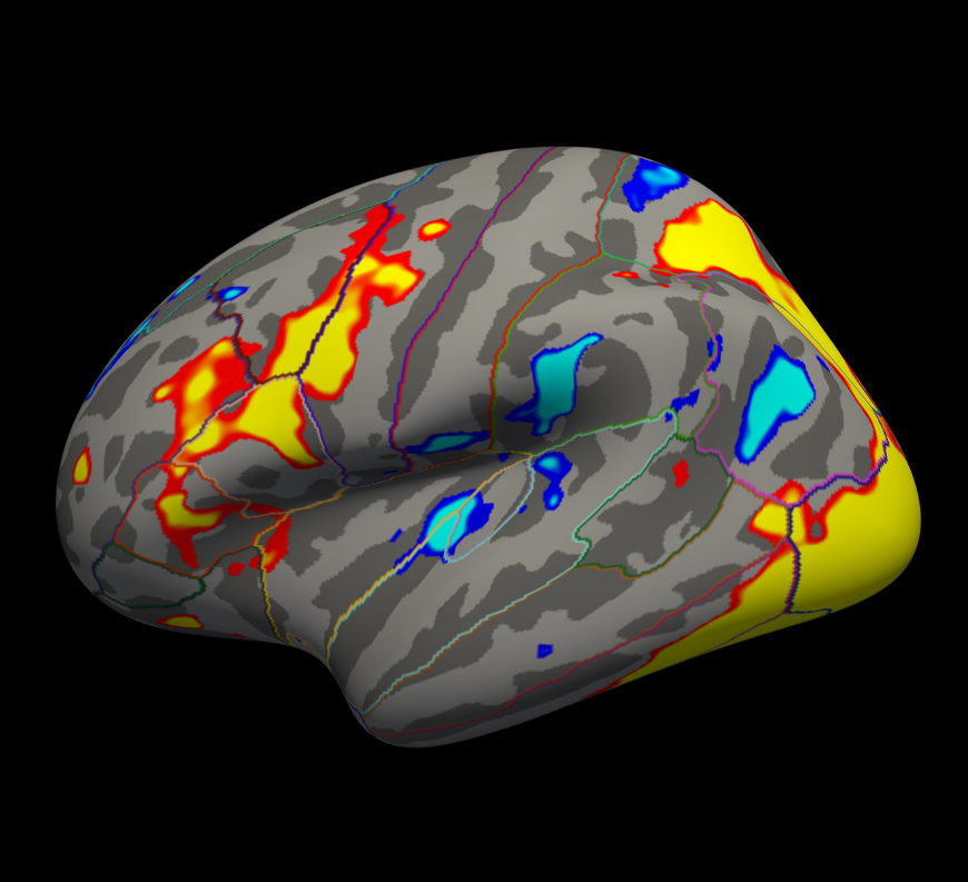
• -fminmax 2 3 : threshold set to 2 (p<.01), saturation to 3 (p<.001)

• Uncorrected p-values
• Positve and negative values

3.2. Correct for Multiple Comparisons

The correction is the same as for the structural group analysis. For example, run:

mri_glmfit-sim --glmdir my-glm --perm 1000 3 pos --cwp .05 --3spaces

• --glmdir my-glm : output from mri_glmfit command
• --perm 1000 3 pos
  • Use permutation simulation

  • Cluster-forming threshold (CFT) of 3 (p<.001)

  • Use positive contrast values

• --cwp .05 : Cluster-wise p-value threshold. Only keep clusters that have p<.05

• --3spaces : correct for a whole brain (ie, lh+rh+subcortical=3spaces) analysis.

• You can also use Permutation Analysis of Linear Models PALM

This will create several outputs in the my-glm/osgm/ directory, though there are three that are most important:

• perm.th30.pos.sig.cluster.summary - cluster summary table (simple ASCII text)
• perm.th30.pos.sig.cluster.nii.gz - overlay with significant clusters
• perm.th30.pos.ocn.annot - annotation of significant clusters
• Name indicates how correction was done (perm, thresh = 3, pos sign)

View the left hemisphere perm.th30.pos.sig.cluster.summary table.

cat my-glm/osgm/perm.th30.pos.sig.cluster.summary

View the clusters on the surface

tksurferfv fsaverage lh inflated \
  -overlay my-glm/osgm/perm.th30.pos.sig.cluster.nii.gz \
  -annot ./my-glm/osgm/perm.th30.pos.sig.ocn.annot -fminmax 1.3 3

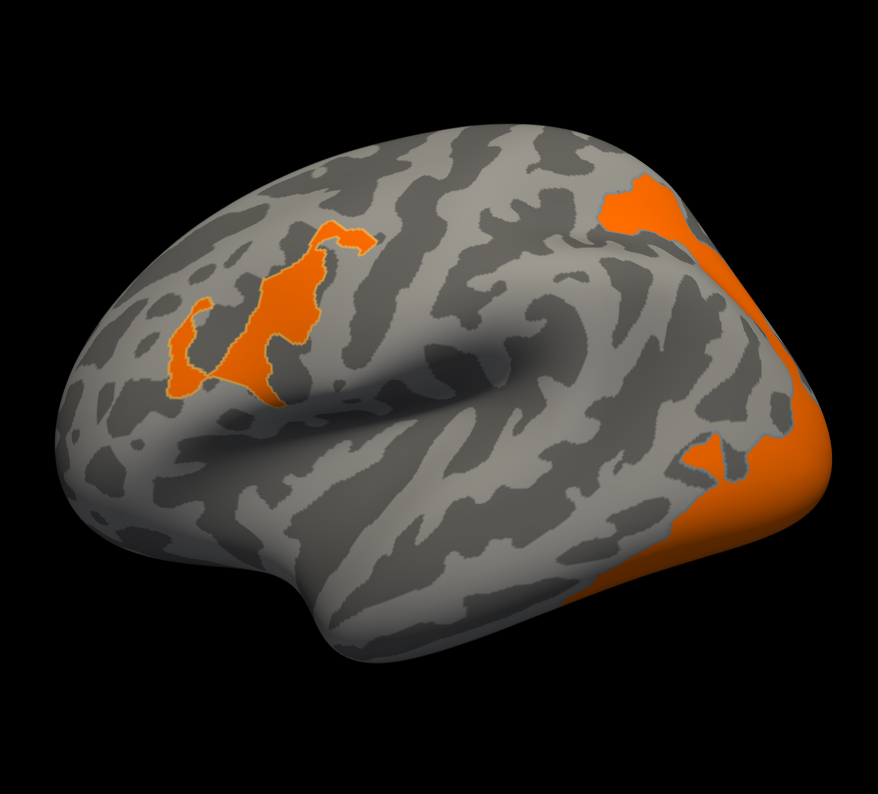
• All clusters are whole-brain corrected at p<.05

• All positive because only positive was selected.
• Annotation gives cluster number

4. Right Hemisphere

Perform the same operations above for the right hemisphere (ie, go into workmem.sm05.rh):

cd $TUTORIAL_DATA/fsfast-functional/group/workmem.sm05.rh/encode-v-base
mri_glmfit --y ces.nii.gz  --osgm \
  --surface fsaverage rh --glmdir my-glm --save-eres --nii.gz

mri_glmfit-sim --glmdir my-glm --perm 1000 3 pos --cwp 0.05 --3spaces

View the right hemisphere perm.th30.pos.sig.cluster.summary table.

cat my-glm/osgm/perm.th30.pos.sig.cluster.summary

5. Subcortical (MNI 305 Space)

Perform the same operations above for the MNI 305 space analysis (ie, go into workmem.sm05.mni305). There are a couple of things that are different about this analysis.

cd $TUTORIAL_DATA/fsfast-functional/group/workmem.sm05.mni305/encode-v-base
ls

This directory has the same files as the surface-based results, though their dimensions are different. All the volumes here are true volumes. The mri_glmfit command is the same as for the surface-based analysis but without the (--surface fsaverage lh) part:

cd $TUTORIAL_DATA/fsfast-functional/group/workmem.sm05.mni305/encode-v-base
mri_glmfit --y ces.nii.gz --osgm  \
  --glmdir my-glm --nii.gz --save-eres
tkmeditfv fsaverage orig.mgz -aparc+aseg -overlay my-glm/osgm/sig.nii.gz -fminmax 2 3

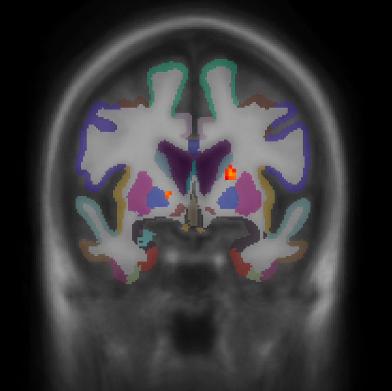
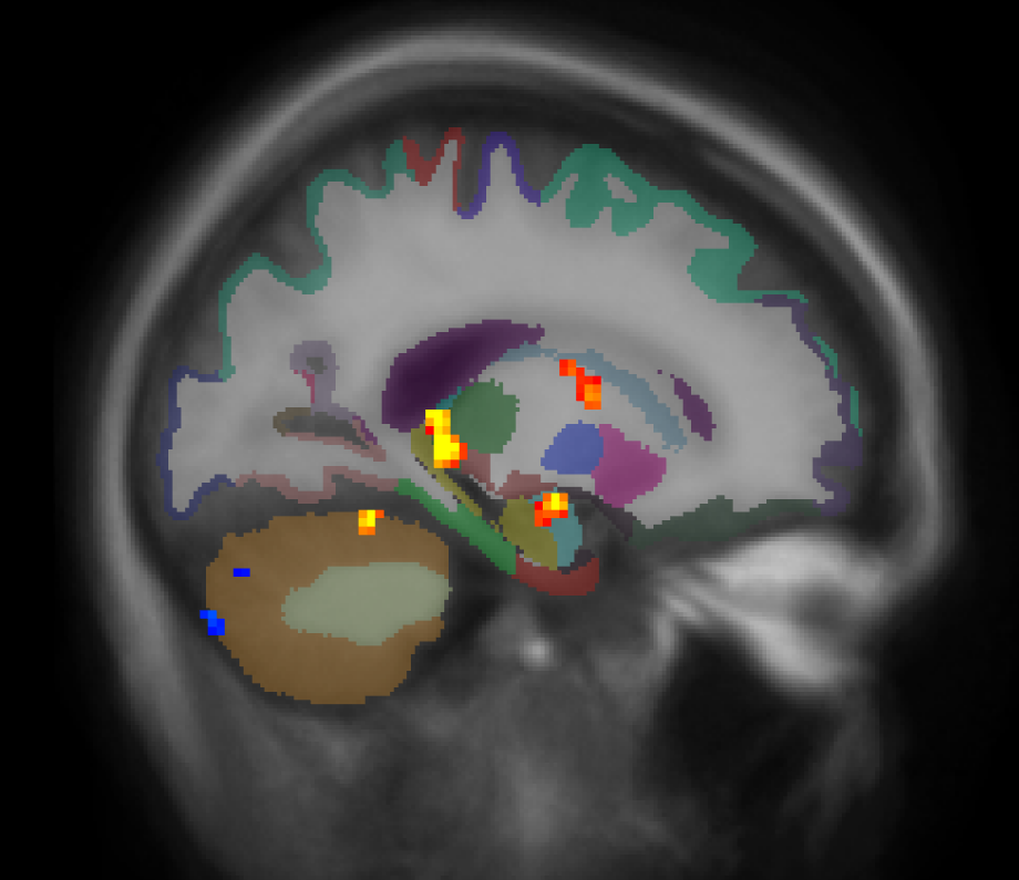
• Left image is coronal slice 54
• Right image is sagittal slice 47
• No activation in cortical areas
• Positive and negative uncorrected p-values

• -fminmax 2 3 : Voxel-wise threshold of 2 (p<.01), color saturation at 3 (p<.001)

To correct the subcortical analysis for multiple comparisons:

mri_glmfit-sim --glmdir my-glm --perm 1000 3 pos --cwp 0.05 --3spaces

• --perm 1000 3 pos :
• Use Permutation

• Cluster-forming threshold (CFT) of 3 (p<.001)

• Use positive contrast values
• As with the surface-based analysis, a summary file is created called perm.th30.pos.sig.cluster.summary
• Creates perm.th30.pos.sig.ocn.nii.gz and perm.th30.pos.sig.ocn.lut. These are segmentations of the clusters.

• You can also use Permutation Analysis of Linear Models PALM

View the subcortical perm.th30.pos.sig.cluster.summary table.

cat my-glm/osgm/perm.th30.pos.sig.cluster.summary

There are five clusters for the subcortical analysis. View the corrected results in the volume:

tkmeditfv fsaverage orig.mgz \
  -ov my-glm/osgm/perm.th30.pos.sig.cluster.nii.gz \
  -seg ./my-glm/osgm/perm.th30.pos.sig.ocn.nii.gz  \
       ./my-glm/osgm/perm.th30.pos.sig.ocn.lut \
  -fminmax 1.3 5

• Only positive values
• p-values are p-values for cluster

• Set threshold to 1.3 (p<.05)

6. Merging the Results

These three tables (which you have already viewed above) give you the clusters across the whole brain for Left Hemisphere, Right Hemisphere, and Subcortical:

cd $TUTORIAL_DATA/fsfast-functional/group
cat workmem.sm05.lh/encode-v-base/my-glm/osgm/perm.th30.pos.sig.cluster.summary
cat workmem.sm05.rh/encode-v-base/my-glm/osgm/perm.th30.pos.sig.cluster.summary
cat workmem.sm05.mni305/encode-v-base/my-glm/osgm/perm.th30.pos.sig.cluster.summary

Merge the corrected results into a single volume for visualization:

vlrmerge --o encode.merged.nii.gz \
  --lh workmem.sm05.lh/encode-v-base/my-glm/osgm/perm.th30.pos.sig.cluster.nii.gz \
  --rh workmem.sm05.rh/encode-v-base/my-glm/osgm/perm.th30.pos.sig.cluster.nii.gz \
  --vol workmem.sm05.mni305/encode-v-base/my-glm/osgm/perm.th30.pos.sig.cluster.nii.gz \
  --scm workmem.sm05.mni305/subcort.mask.nii.gz

Creates encode.merged.nii.gz by mapping the left and right hemispheres to the volume and merging with the subcortical results. Subcortical results are limited to subcortical regions because of the subcortical mask (-scm) applied. View the merged volume:

tkmeditfv fsaverage orig.mgz -aparc+aseg -ov encode.merged.nii.gz -fminmax 1.3 5 -surfs

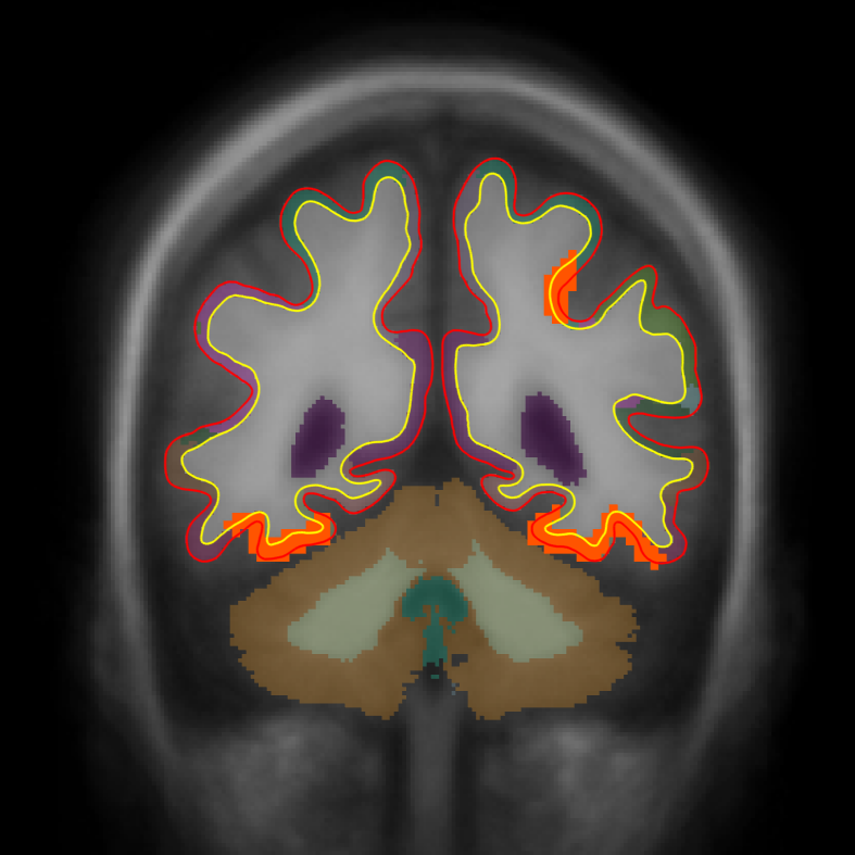
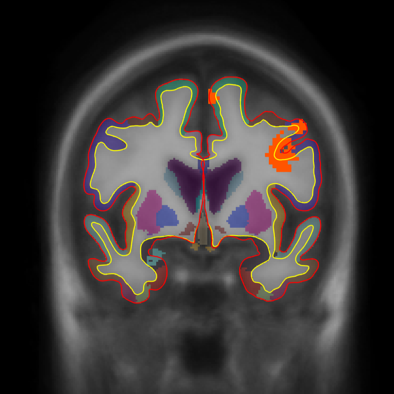
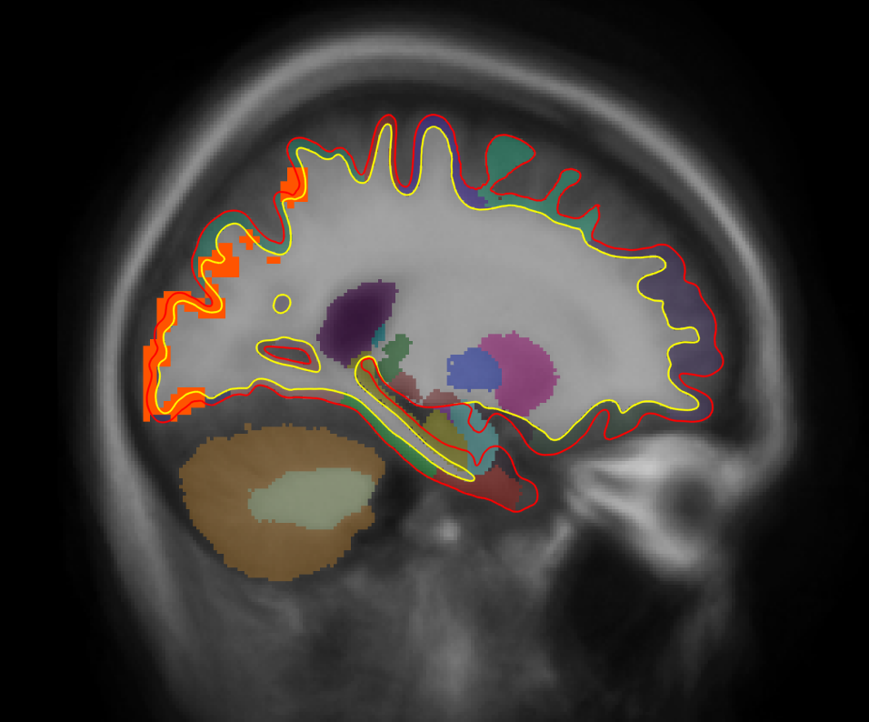
• Left image is coronal slice 30
• Middle image is coronal slice 54
• Right image is sagittal slice 25
• Color indicates cluster p-value.
• All positive because only positive was selected.
• Cortical activation comes from the cortical analysis
• Subcortical activation comes from the subcortical analysis

• All activation in this image has been corrected for whole-brain multiple comparisons at p<.05.

7. Quiz

You can test your knowledge of part 2 of the FS-FAST tutorial by clicking here for a quiz!

Back to list of all tutorials | Back to course page | Previous (First Level Analysis)