• MultivariateStatisticalAnalysisDMRI

Multivariate statistical analysis of diffusion imaging parameters using partial least squares: Applications to white matter variations in Alzheimer's disease

Ender Konukoglu, Jean-Philippe Coutu, David H. Salat and Bruce Fischl, Neuroimage 2016 134:573-586

This page describes the software tool released as a part of the article published in Neuroimage (doi:10.1016/j.neuroimage.2016.04.038) . The tool is written in python and can be used on different platforms. We have tested the tool in Linux (CentOS 6.7) and Mac OS (Yosemite).

Requirements:

The software requires basic installation of numpy and scipy. In addition to these it also requires nibabel (http://nipy.org/nibabel/) to be able to read/write Nifti images.

The most convenient way to use to tool is to set up a python environment using one of the available scientific environments such as:

• Anaconda (https://www.continuum.io/downloads)

• Enthought (https://store.enthought.com/downloads/#default)

Once one of these environments is set up, you can install nibabel simply by executing the command:

• pip install nibabel

on a terminal.

Installation:

After setting up the python environment you can set up the tool by downloading the tar-ball and extracting it in a directory of your choice.

The tar-ball contains the following:

• MultivariateProcedures.py

• MultivariateDMRIAnalysis.py
• run_dev.csh
• example_data/
• example_output/

The python files contain the tool itself. The run_dev.csh file provides example terminal commands on how to run the different types of analysis using the example data provided in the example_data folder. example_output folder is the typical outputs one can expect to get by running the commands in run_dev.csh file.

Analysis:

The article presents three different types of analysis which can all be run using the software tool described here. The different types of analyses and the corresponding sections in the articel are:

1. Multivariate group analysis (Section 2.2)
2. Comparing multivariate effect types of different conditions (Section 2.4)
3. Regressing out nuissance parameters in the multivariate setting (Section 2.5)

The basic command to get help on how to run the tool is

• python MultivariateProcedures.py

or

• python MultivariateProcedures.py -h

Basic usage with the the available options are:

• python MultivariateProcedures.py -d image1 image2 ... -s data_shape -g group_file -a age_file -t type_of_analysis[group(default)|regressing_out|effect_comparison|aging] -tfce tfce_flag[0(default)|1] -fdr fdr_flag[0(default)|1] -fdr_alpha alpha[0.1(default)] -nperm number_of_permutation[2000(default)] -o output_file_prefix -otype output_type[txt(default)|binary] -pth pvalue_threshold_negLog10[2(default)] -rth region_threshold[0.1(default)] -tract

Different options are:

• -d : list of images. different modalities are given as separate files. each image file is a matrix of numPoints x numSamples. numPoints is the total number of points in the image. Even if only a certain part of the image has non-zero values please provide the entire image. Internally such regions are detected and analysis is not performed. txt or csv files are accepted. if csv do not use "," as delimiter.
• -s : data shape. this is a series of integers indicating the shape of the image or volume. two numbers are given if 2D image and 3 if the image is a volume, e.g. 100 100 (for a 100x100 2D image)
• -g : group file. this is a txt file indicating labels, as integers, for each subject in the sample. in the label file 0 corresponds to controls and 1 to the group of interest. For effect_type analysis one also needs to provide label 2 for the 2nd group of interest.
• -a : age file. this is a txt file indicating ages or another continuous variable for each subject
• -t : type of analysis. options are group (for basic group comparison), aging (for continuous valued analysis such as aging), regressing_out (group comparison with regressing out nuissance continuous parameter age), effect_comparison (comparing effects of different conditions as given with different labels in the group file)
• -tfce : 0 or 1. Flag to perform TFCE enhancement. TFCE is only available when the measurements form a volume, 2D image or a tract. If volume then data shape parameter should have 3 components, if 2D image 2 components and if tract then only one component AND -tract option should be enabled.
• -fdr : 0 or 1. flag to perform FDR correction
• -fdr_alpha : alpha value of the FDR correction
• -nperm : number of permutations using the statistical test, e.g. 1000
• -o : prefix of the output file. the actual file names depend on the analysis
• -otype : binary or txt. type of the output file. if binary the images are written down in binary and should be read as such. the images are written row-major (C-format)

• -pth : a floating point number. threshold for the -log_10(pvalue). default value is 2, which corresponds to p < 0.01.

• -rth : a region threshold to constraint the effect-comparison analysis to the areas where both conditions are significant. threshold is on the probability
• -tract : flag to indicate whether the data is a tract or 1D data with spatial context in it. Default is false and when -tract is given it is set as true and TFCE in 1D becomes available.

Examples

We will demonstrate the software tool for different analysis using the data provided in example_data folder. This folder contains a sample dataset used in the synthetic experiments presented in the supplementary material to the main article. The folder contains

• labels.txt - label file composed of three groups indicated with 0 (CN), 1 and 2 (two different disease groups). Contains 300 values in a row.
• ages.txt - ages for the synthetic subjects. Contains 300 values in a row.
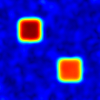
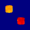
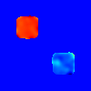
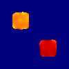
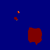
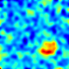
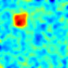
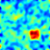
• features_0.txt, features_1.txt, features_2.txt - three different parametric maps similar to the analyses presented in the article. Each file contains a table of 10000 x 300 values, which corresponds to 10000 measurements from 300 subjects. Each column corresponds to one subject's measurements and corresponds to a 100 x 100 image. The images are formed into a vector in a row-major format. The example images are as:

  

Multivariate Group Analysis for Group Differences

The first analysis is to detect group differences between controls (label = 0) and disease (label = 1). We run the following code to perform this analysis:

• python MultivariateProcedures.py -d example_data/features_0.txt example_data/features_1.txt example_data/features_2.txt -g example_data/labels.txt -t group -s 100 100 -o ./example_output/group_comparison_ -tfce 1 -fdr 1

Notice that this command performs TFCE enhancement and FDR correction for multiple comparisons problem. The outputs of this analysis are saved in the example_output folder with the prefix group_comparison_:

• example_output/group_comparison_data_info.txt : holds the image dimensions and the number of channels in a row vector (100, 100, 3)
• example_output/group_comparison_vectors_th_0.txt : the first component of the effect type in a row vector with 10000 components. it corresponds to an image of 100x100 saved in a row-major format. values are only shown in the regions where the effect strength is statistically significant (from the thresholded p_value map).
• example_output/group_comparison_vectors_th_1.txt : the second component of the effect type
• example_output/group_comparison_vectors_th_2.txt : the third component of the effect type
• example_output/group_comparison_covariance_strength.txt : effect strength - covariance - in a row vector with 10000 components.
• example_output/group_comparison_pvals_covariance.txt : p-value map as a vector with 10000 components.
• example_output/group_comparison_pvals_covariance_th.txt : thresholded p-value map as a vector 10000 components.

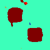
The data_info.txt file is saved to keep the information necessary to convert the results to images (shape of the multidimensional array). Below we show the output images for effect strength, thresholded p-value maps and the three components of the effect-types:

Multivariate Group Analysis for Aging Effects

The tool can also be used to perform group analysis for continuous variables. Here we provide an example for the aging analysis. We run the following command to perform the analysis:

• python MultivariateProcedures.py -d example_data/features_0.txt example_data/features_1.txt example_data/features_2.txt -a example_data/ages.txt -t aging -s 100 100 -o ./example_output/continuous_value_ -tfce 1 -fdr 1 -otype binary

Notice that this time the output type is given as binary hence the output files are written in binary. To read the binary files one can use the following steps in python for reading the vectors:

1. import numpy as np
2. fid = open('example_output/continuous_value_vectors_th.dat', 'r')
3. V = np.fromfile(fid)
4. fid.close()

The outputs of this analysis are:

• example_output/continuous_value_data_info.txt - same as before.
• example_output/continuous_value_covariance_strength.dat - same as before but written as a binary file.
• example_output/continuous_value_pvals_covariance.dat - same as before
• example_output/continuous_value_pvals_covariance_th.dat - same as before
• example_output/continuous_value_vectors_th.dat - a file with 30000 values. different components of the effect-types are written in one file. Each component is written one after the other. To reshape into a easy to visualize format do a reshape, i.e. W = V.reshape([3,100,100]).

Regressing out nuissance parameters in the multivariate setting

The tool allows using the method explained in Section 2.5 of the main article. For the example data we run the following code:

• python MultivariateProcedures.py -d example_data/features_0.txt example_data/features_1.txt example_data/features_2.txt -g example_data/labels.txt -a example_data/ages.txt -t regressing_out -s 100 100 -o ./example_output/group_comparison_minusAge_ -nperm 1000 -otype binary -pth 1.3 -tfce 1 -fdr 1

This analysis regresses out the effects of age - as given in the ages.txt file - and then computes group differences between label = 0 and label = 1 groups. The group differences are given both for the "parallel component" and the "orthogonal component". We see that this time the p-value threshold is set to 1.3 which corresponds to p < 0.05.

• example_output/group_comparison_minusAge_data_info.txt
• example_output/group_comparison_minusAge_orth_covariance_strength.dat
• example_output/group_comparison_minusAge_orth_pvals_covariance.dat
• example_output/group_comparison_minusAge_orth_pvals_covariance_th.dat
• example_output/group_comparison_minusAge_orth_vectors_th.dat
• example_output/group_comparison_minusAge_par_covariance_strength.dat
• example_output/group_comparison_minusAge_par_pvals_covariance.dat
• example_output/group_comparison_minusAge_par_pvals_covariance_th.dat

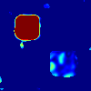
The structures of the files are similar to previous examples. We observe that there is no effect type results for the parallel component as this is unnecessary. The thresholded p value maps for the parallel and orthogonal components are as shown below:

Comparing effect types between two conditions

The last example shows how to use the software to compare multivariate effect types between two conditions. The conditions are indicated in the label.txt file as label=0 - controls, label = 1 condition 1 and label=2 condition 2. We run the following command to perform the analysis:

• python MultivariateProcedures.py -d example_data/features_0.txt example_data/features_1.txt example_data/features_2.txt -g example_data/labels.txt -a example_data/ages.txt -t effect_comparison -s 100 100 -o ./example_output/ -otype txt -nperm 1000 -rth 0.1

Notice the extra variable -rth which sets the regional threshold described previously and also in the main article. The outputs of this analysis are:

• example_output/effect_type_diff_pvals.txt - p value maps for the difference in effect type. 10000 values which correspond to 100x100 images.
• example_output/effect_type_diff_pvals_th.txt - thresholded p value maps for the difference in effect type

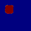
Both results are given below as images. First the p value maps and then the thresholded maps at pth = 2: