|
Size: 27
Comment:
|
← Revision 106 as of 2026-11-03 14:05:11 ⇥
Size: 17216
Comment:
|
| Deletions are marked like this. | Additions are marked like this. |
| Line 1: | Line 1: |
| Describe PhotoTools here. | = Photo Reconstruction Documentation = <<TableOfContents>><<BR>><<BR>> == Citation == If you use these tools in your analysis, please cite: * Gazula, H., Tregidgo, H.F., Billot, B., Balbastre, Y., Williams Ramirez, J., Herisse, R., Deden-Binder, L.J., Casamitjana, A., Melief, E.J., Latimer, C.S. and Kilgore, M.D., 2024. Machine learning of dissection photographs and surface scanning for quantitative 3D neuropathology. Elife, 12, p.RP91398. [[https://doi.org/10.7554/eLife.91398.4|doi]] The machine learning slice imputation in the reconstruction is described in: * Crespo-Aguirre, M., Williams-Ramirez, J., Zemlyanker, D., Hu, X., Deden-Binder, L.J., Herisse, R., Montine, M., Connors, T.R., Mount, C., !MacDonald, C.L., Keene, C.D., Latimer, C.S., Oakley, D.H., Hyman, B.T., Lawry-Aguila, A. and Iglesias, J.E., 2026. Improving neuropathological reconstruction fidelity via AI slice imputation. Acta Neuropathologica Communications. [[https://doi.org/10.1186/s40478-026-02451-3|doi]] Automatic segmentation model trained using nnUNet: * Williams Ramirez, J., Zemlyanker, D., Deden-Binder, L., Herisse, R., Garcia Pallares, E., Gopinath, K., Gazula, H., Mount, C., Kozanno, L.N., Marshall, M.S., Connors, T.R., Frosch, M.P., Montine, M., Oakley, D.H., Mac Donald, C.L., Keene, C.D., Hyman, B.T., Fischl, B. and Iglesias, J.E., 2026. A public generalizable AI tool for automated segmentation of coronal brain tissue slabs for 3D neuropathology. PLOS One, 21(8), p.e0355740. [[https://doi.org/10.1371/journal.pone.0355740|doi]] * Isensee, F., Jaeger, P.F., Kohl, S.A., Petersen, J. and Maier-Hein, K.H., 2021. nnU-Net: a self-configuring method for deep learning-based biomedical image segmentation. Nature methods, 18(2), pp.203-211. [[https://www.youtube.com/watch?v=wo5meYRaGUY|Click here for a video with an overview of the method]]<<BR>> {{attachment:video_screenshot.png||width="666"}} <<BR>><<BR>> == Purpose == This manual provides an end-to-end guide for using the tools available in FreeSurfer to reconstruct dissection photographs of brain slabs into a 3D reconstruction for quantitative analysis. Reconstructions are done by registering photographs to a 3D reference such as an MRI, a post-mortem surface scan, or an atlas. The guide covers acquiring surface scans prior to slabbing, photographing tissue slabs, and preprocessing photographs using the dissection_photo graphical user interface.<<BR>><<BR>> == Requirements == * The latest FreeSurfer development version sourced in your terminal. * Model files (downloaded once): * the [[https://ftp.nmr.mgh.harvard.edu/pub/dist/lcnpublic/dist/dissection_photo_model/photo_imputation_unet.pth|reconstruction model]], downloaded into `$FREESURFER_HOME/models` * A CUDA-enabled graphics card is optional: segmentation and reconstruction are much faster with one. == Overview == 1. '''Acquire a 3D reference''': either a surface scan or an MRI. Without one, slabs are registered to an atlas. 1. '''Photograph the tissue slabs''' 1. '''Preprocess the photos in the dissection photo GUI''' 1. '''Reconstruct the 3D volume''' 1. '''Downstream analysis of photographs''' = Part 1: Acquisition = == Surface scanning == A surface scan of the specimen is taken after the cerebellum has been sectioned off and before the specimen is slabbed. The full scanning protocol is available on its own page: '''[[PhotoTools Surface Scanning|Surface Scanning Protocol]]'''. Summary of the key requirements of a reference mesh: * The cerebellum removed: it is not on the slabs, so including it in the scan leads to an incorrect reconstruction. * The sides of the specimen captured. * A watertight mesh, saved as `.stl`. Small holes in the initial point cloud due to deep sulci are fine; these will be covered by the meshing process. <<BR>> == Photographing the slabs == The slab photography protocol (background, tissue placement, lighting, and the markers used for pixel and perspective correction) is on its own page: '''[[PhotoTools Slab Photography|Slab Photography Protocol]]'''. Summary of the key requirements of a slab photograph: * A uniform, high-contrast background (for example solid black), so the tissue is easy to segment. * All slabs photographed from the same side, anterior or posterior. Posterior photographs need the flag '''--photos_of_posterior_side''' in the final reconstruction command. * Detached pieces of a slab placed as close to their original anatomical position as possible. * Landmarks of known distance in every photograph: at minimum a ruler, preferably the four printed fiducial markers at the corners of a rectangle of known size, with all tissue inside that rectangle. * Consistent lighting across all slabs. <<BR>> = Part 2: Preprocessing Photographs with the Dissection Photo App = The dissection photo app has five principal windows for each subject: '''Add photos''', '''Correction''', '''Segmentation''', '''Connected components''' and '''Reconstruction'''. The step bar at the top of the window shows which step is being done. Users can backtrack by clicking any of the previous steps at any time, or click the house icon to return to the Projects screen with a summary of all reconstructions done or in process. For each project, work is saved as you go, so the app can be closed at any time and you can pick up later where you left off. Before continuing, make sure the development version of FreeSurfer is properly sourced, you have downloaded the model weights, and have set '''NNUNET_MODEL_DIR''' as an environment variable pointing to the segmentation model. To start the application, use the command '''dissection_photo_2'''. <<BR>> == Projects Page == Each specimen corresponds to a '''project''': a folder which will be populated with the outputs from all steps. The project home contains a summary of all projects and their progress. {{attachment:ds2_00_projects.png||width="560"}} <<BR>> ''Projects Home screen.'' * To start processing a new batch of dissection photographs click on '''New Project'''. * Open a project to continue where you left off or backtrack to any completed steps. '''Tip:''' For advanced users, the gear icon can be used to change which resources are used by the automatic segmentation model, covered in [[#Automatic_Segmentation_Settings|automatic segmentation settings]]. After naming a project you will be prompted to save a folder of the same name. It is in this folder that the outputs of all steps will be stored. == Directory Structure == For each project the following directory structure will be populated with all outputs. ||Folder / file ||Contents || ||`photos/` ||Copy of the original photographs || ||`deformed/` ||Pixel-corrected photos || ||`mask/` ||Binary tissue masks || ||`connected_components/` ||Label maps per slab || ||`recon/` ||The 3D-photo reconstruction || == Step 1. Add photographs == 1. Drag and drop a folder containing dissection photographs, or click '''Upload Images'''. 1. Select the photographs that should be used for the reconstruction. This can be used to omit repeat photographs, dissection photographs of cerebellar tissue, or gross photographs done prior to slabbing. Double click on any image in the grid for a larger preview. 1. If you have or would like to create a calibration file to automate pixel correction, click on '''+ Add a calibration file (optional)''' and follow the steps in [[#Optional:_Making_a_calibration_file|Making a Calibration File]] and then [[#Prospective_Correction_.28Using_fiducial_markers_and_calibration_file.29|Prospective Correction]]. 1. Click '''Get started'''. ||<:> {{attachment:ds2_01_add_photos_empty.png||width="420"}} <<BR>> ''Add photos, before any photographs are chosen.'' ||<:> {{attachment:ds2_02_add_photos_populated.png||width="420"}} <<BR>> ''Photographs added, with the calibration file box expanded.'' || === Optional: Making a calibration file === This step only needs to be done once, as long as the markers are not moved. For more information on proper usage refer to the [[PhotoTools Slab Photography#Markers_for_pixel_and_perspective_corrections|Markers for pixel and perspective corrections]] section of the slab photography page. 1. On the Add photos menu, click '''+ Add a calibration file (optional)''' to expand the calibration file box, and click on '''Create one''' under the Upload Calibration button. 1. On the next menu, if you have not printed out the fiducial markers, they can be downloaded for printing by clicking the '''Download Marker Printout''' button. 1. Next, place markers at a known distance in a rectangle formation on the photography table. Be sure that opposite sides of the rectangle created by the fiducial markers are parallel; inaccurate marker placement can lead to incorrect perspective correction. 1. Upload the photograph of the empty dissection table with just the markers present, and enter the width and height of the fiducial box. 1. For each of the markers, click its centre and outer circle. Options to zoom, pan, and redo/undo can help fix mistakes and make the best calibration possible. 1. Click '''Save Calibration''' and save your calibration file in an easy-to-access location. '''Tip:''' Because of slight lens distortion, the overlaid labels for the outer circle of the markers might not always align throughout the whole circumference. This is not an issue. {{attachment:ds2_03_calibration_photo.png||width="640"}} <<BR>> ''The photograph of the empty table with the four markers, uploaded.'' ||<:> {{attachment:ds2_04_calibration_zoomed.png||width="420"}} <<BR>> ''Zoomed in on one marker, before clicking.'' ||<:> {{attachment:ds2_05_calibration_clicks.png||width="420"}} <<BR>> ''The marker's centre and outer circle clicked.'' || == Step 2: Pixel Correction == This step corrects all photographs to be at the same pixel size. Additionally, it can correct for perspective when using a calibration file, or when doing manual correction in 4-point mode. === Prospective Correction (Using fiducial markers and calibration file) === * Every photo is corrected automatically as soon as Correction opens. The markers are found in each photo separately, so it does not matter if the camera moved between photos. * Check each photo: '''Original''' shows the photo as taken, with the marker centres that were found; '''Corrected''' shows the result. A green tick in the strip at the bottom marks each corrected photo. * If the markers cannot be found in a photo, the app says which ones. On each of them, click the centres of the four markers on the Original view and click '''Correct this photo'''. === Retrospective Correction (Using a spatial reference within the photographs) === Choose how many points you can mark, enter the real distances, and place the points on each photo: ||'''Mode'''||'''You need'''||'''Corrects'''|| ||2 Point||One ruler or other known distance (entered as '''Ruler width (mm)''')||Pixel size only|| ||3 Point||Three corners of a rectangle, e.g. two rulers at right angles||Pixel size, approximate perspective|| ||4 Point||Four corners of a rectangle||Pixel size and perspective|| * Ctrl + left click places a point; once all are placed, Ctrl + click moves the nearest one. '''Clear points''' starts again. * Click '''Correct this photo''' (Ctrl + W also moves on to the next photo). Place points on the Original view; the Corrected view is for checking. ||<:> {{attachment:ds2_06_correction_ruler.png||width="420"}} <<BR>> ''2 Point mode: two points placed along a 150 mm ruler (Original).'' ||<:> {{attachment:ds2_07_correction_done.png||width="420"}} <<BR>> ''The corrected photo, with rulers (Corrected).'' || When every photo is corrected, make sure to click '''Continue to Segmentation'''. == Step 3: Binary Segmentation == While you were correcting, the app was already finding the tissue in each corrected photo. Here you check each mask and fix it. ||<:> {{attachment:ds2_08_segmentation_mask_on.png||width="440"}} <<BR>> ''The automatic mask (green) shown over the slabs.'' ||<:> {{attachment:ds2_09_segmentation_mask_off.png||width="346"}} <<BR>> ''The mask hidden ('''Show mask''' off); the note at the top lists the masks not yet previewed.'' || * '''Brush''' (Q) adds to the mask, '''Eraser''' (W) removes from it, and '''Fill''' (E) fills an area. Apply the tool with Ctrl + left drag; set the sizes with the sliders. * '''Mask opacity''' changes how see-through the mask is; '''Show mask''' (Ctrl + T) hides and shows it. Undo and redo with Ctrl + Z and Ctrl + Shift + Z. * Leave out everything that is not slab tissue: the background, labels, and fragments that do not belong to a slab. * '''IMPORTANT''': the cortical surface should not be part of the masks, so the first slab (if photographed from the anterior side) or the last slab (if photographed from the posterior side) should '''NOT''' be included. * You need to look at every photo's mask before '''Continue to Connected Components''' becomes available; a note at the top says which ones are left. === Automatic Segmentation Settings === Open them from the gear on the Projects screen. Changes apply the next time photos are segmented. {{attachment:ds2_10_seg_settings.png||width="480"}} <<BR>> ''Automatic segmentation settings.'' ||'''Setting'''||'''What it does'''|| ||Automatic segmentation (On / Off)||Off: every mask is drawn by hand from scratch. Only turn it off if the automatic segmentation fails on your photos.|| ||Model folds||Automatic: 5 folds on a GPU, 1 on the CPU. Five folds are steadier but 4-5x slower.|| ||Run on||Automatic uses the GPU if there is one; or choose GPU or CPU.|| ||Maximum threads||The most processor threads segmentation may use. If the computer has fewer, it uses all it has.|| ||Model folder||The folder of the segmentation model (`nnUNetTrainer__nnUNetPlans__2d`).|| == Step 4: Slab Connected Components == Here you tell the app which pieces of tissue belong to which slab. * In each photo, draw a box inside each slab (Ctrl + left drag), always in the same order: anterior to posterior, or posterior to anterior. The slab is colored as soon as its box is drawn. * Keep boxes small and inside the tissue, and do not let them overlap. If a slab is in several pieces (e.g. a detached temporal lobe), make sure its box touches every piece. * Click '''Save components''' (Ctrl + W also moves on to the next photo); moving to another photo saves it too. A green tick marks saved photos. If you change a saved photo, its tick goes away until you save it again. * Undo and redo with Ctrl + Z and Ctrl + Shift + Z. '''Slab overlay''' changes how strongly the slabs are colored. {{attachment:ds2_11_components_empty.png||width="420"}} <<BR>> ''Before any boxes are drawn.'' ||<:> {{attachment:ds2_12_components_good.png||width="420"}} <<BR>> ''One small box inside each slab; each slab is colored and the photo is saved.'' ||<:> {{attachment:ds2_13_components_bad.png||width="420"}} <<BR>> ''How '''NOT''' to draw boxes: they overlap each other and cover background.'' || == Step 5: Photo Reconstruction == Please see our separate page on the command [[mri_3d_photo_recon]]. The last step runs [[mri_3d_photo_recon]] on the images of the project. While the reconstruction is running in the background the user can continue processing images of other cases. 1. '''Output folder''': the folder inside the project for the results (default `recon`). 1. '''Slabs''': the hemisphere, the slab thickness in mm, which face of the slabs was photographed (anterior or posterior), the order the photos were taken in, and whether the tissue is fixed or fresh. 1. '''Reference''': none (the MNI atlas), a surface mesh (`.stl`), an MRI scan, or both. See [[#Which_reference_should_I_use.3F|Which reference should I use?]] 1. Optionally: the number of threads, a graphics card, and the advanced settings. Empty expert weights use the command's own defaults, shown in grey. 1. Click '''Run Reconstruction'''. The command being run is shown on the right ('''Copy command''' copies it, for example to run it on another computer), and its output appears in the log below it. The reconstruction keeps running if you switch to another project; the Projects screen shows its progress. {{attachment:ds2_14_reconstruction.png||width="640"}} <<BR>> ''A reconstruction running, with the command and its log.'' <<BR>> = Part 3: Downstream Tasks = == Photo-Synthseg Segmentation == The 3D reconstructed stacks can be segmented with SynthSeg using the flag --photo. Please see [[https://surfer.nmr.mgh.harvard.edu/fswiki/SynthSeg|the wiki page for SynthSeg]] for further information. || {{attachment:43_synthseg_photo.jpg||height="400"}} || {{attachment:44_synthseg_parc.jpg||height="400"}} || '''Example for running SynthSeg on a Left Hemisphere''' <<BR>> . mri_synthseg \ ''''' ''''' . --i ./recon/photo_recon.mgz \ ''''' ''''' . --o ./recon/photo_recon_synthseg.mgz \ ''''' ''''' . --photo left \ ''''' ''''' . --parc ''''' ''''' |
Photo Reconstruction Documentation
Contents
- Photo Reconstruction Documentation
- Part 1: Acquisition
- Part 2: Preprocessing Photographs with the Dissection Photo App
- Part 3: Downstream Tasks
Citation
If you use these tools in your analysis, please cite:
Gazula, H., Tregidgo, H.F., Billot, B., Balbastre, Y., Williams Ramirez, J., Herisse, R., Deden-Binder, L.J., Casamitjana, A., Melief, E.J., Latimer, C.S. and Kilgore, M.D., 2024. Machine learning of dissection photographs and surface scanning for quantitative 3D neuropathology. Elife, 12, p.RP91398. doi
The machine learning slice imputation in the reconstruction is described in:
Crespo-Aguirre, M., Williams-Ramirez, J., Zemlyanker, D., Hu, X., Deden-Binder, L.J., Herisse, R., Montine, M., Connors, T.R., Mount, C., MacDonald, C.L., Keene, C.D., Latimer, C.S., Oakley, D.H., Hyman, B.T., Lawry-Aguila, A. and Iglesias, J.E., 2026. Improving neuropathological reconstruction fidelity via AI slice imputation. Acta Neuropathologica Communications. doi
Automatic segmentation model trained using nnUNet:
Williams Ramirez, J., Zemlyanker, D., Deden-Binder, L., Herisse, R., Garcia Pallares, E., Gopinath, K., Gazula, H., Mount, C., Kozanno, L.N., Marshall, M.S., Connors, T.R., Frosch, M.P., Montine, M., Oakley, D.H., Mac Donald, C.L., Keene, C.D., Hyman, B.T., Fischl, B. and Iglesias, J.E., 2026. A public generalizable AI tool for automated segmentation of coronal brain tissue slabs for 3D neuropathology. PLOS One, 21(8), p.e0355740. doi
- Isensee, F., Jaeger, P.F., Kohl, S.A., Petersen, J. and Maier-Hein, K.H., 2021. nnU-Net: a self-configuring method for deep learning-based biomedical image segmentation. Nature methods, 18(2), pp.203-211.
Click here for a video with an overview of the method

Purpose
This manual provides an end-to-end guide for using the tools available in FreeSurfer to reconstruct dissection photographs of brain slabs into a 3D reconstruction for quantitative analysis. Reconstructions are done by registering photographs to a 3D reference such as an MRI, a post-mortem surface scan, or an atlas. The guide covers acquiring surface scans prior to slabbing, photographing tissue slabs, and preprocessing photographs using the dissection_photo graphical user interface.
Requirements
The latest FreeSurfer development version sourced in your terminal.
- Model files (downloaded once):
the reconstruction model, downloaded into $FREESURFER_HOME/models
- A CUDA-enabled graphics card is optional: segmentation and reconstruction are much faster with one.
Overview
Acquire a 3D reference: either a surface scan or an MRI. Without one, slabs are registered to an atlas.
Photograph the tissue slabs
Preprocess the photos in the dissection photo GUI
Reconstruct the 3D volume
Downstream analysis of photographs
Part 1: Acquisition
Surface scanning
A surface scan of the specimen is taken after the cerebellum has been sectioned off and before the specimen is slabbed. The full scanning protocol is available on its own page: Surface Scanning Protocol.
Summary of the key requirements of a reference mesh:
- The cerebellum removed: it is not on the slabs, so including it in the scan leads to an incorrect reconstruction.
- The sides of the specimen captured.
A watertight mesh, saved as .stl. Small holes in the initial point cloud due to deep sulci are fine; these will be covered by the meshing process.
Photographing the slabs
The slab photography protocol (background, tissue placement, lighting, and the markers used for pixel and perspective correction) is on its own page: Slab Photography Protocol.
Summary of the key requirements of a slab photograph:
- A uniform, high-contrast background (for example solid black), so the tissue is easy to segment.
All slabs photographed from the same side, anterior or posterior. Posterior photographs need the flag --photos_of_posterior_side in the final reconstruction command.
- Detached pieces of a slab placed as close to their original anatomical position as possible.
- Landmarks of known distance in every photograph: at minimum a ruler, preferably the four printed fiducial markers at the corners of a rectangle of known size, with all tissue inside that rectangle.
- Consistent lighting across all slabs.
Part 2: Preprocessing Photographs with the Dissection Photo App
The dissection photo app has five principal windows for each subject: Add photos, Correction, Segmentation, Connected components and Reconstruction. The step bar at the top of the window shows which step is being done. Users can backtrack by clicking any of the previous steps at any time, or click the house icon to return to the Projects screen with a summary of all reconstructions done or in process. For each project, work is saved as you go, so the app can be closed at any time and you can pick up later where you left off.
Before continuing, make sure the development version of FreeSurfer is properly sourced, you have downloaded the model weights, and have set NNUNET_MODEL_DIR as an environment variable pointing to the segmentation model. To start the application, use the command dissection_photo_2.
Projects Page
Each specimen corresponds to a project: a folder which will be populated with the outputs from all steps. The project home contains a summary of all projects and their progress.
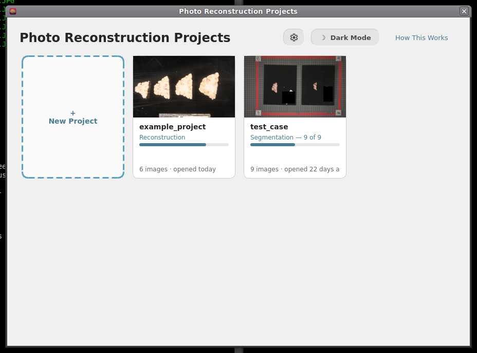
Projects Home screen.
To start processing a new batch of dissection photographs click on New Project.
- Open a project to continue where you left off or backtrack to any completed steps.
Tip: For advanced users, the gear icon can be used to change which resources are used by the automatic segmentation model, covered in automatic segmentation settings.
After naming a project you will be prompted to save a folder of the same name. It is in this folder that the outputs of all steps will be stored.
Directory Structure
For each project the following directory structure will be populated with all outputs.
Folder / file |
Contents |
photos/ |
Copy of the original photographs |
deformed/ |
Pixel-corrected photos |
mask/ |
Binary tissue masks |
connected_components/ |
Label maps per slab |
recon/ |
The 3D-photo reconstruction |
Step 1. Add photographs
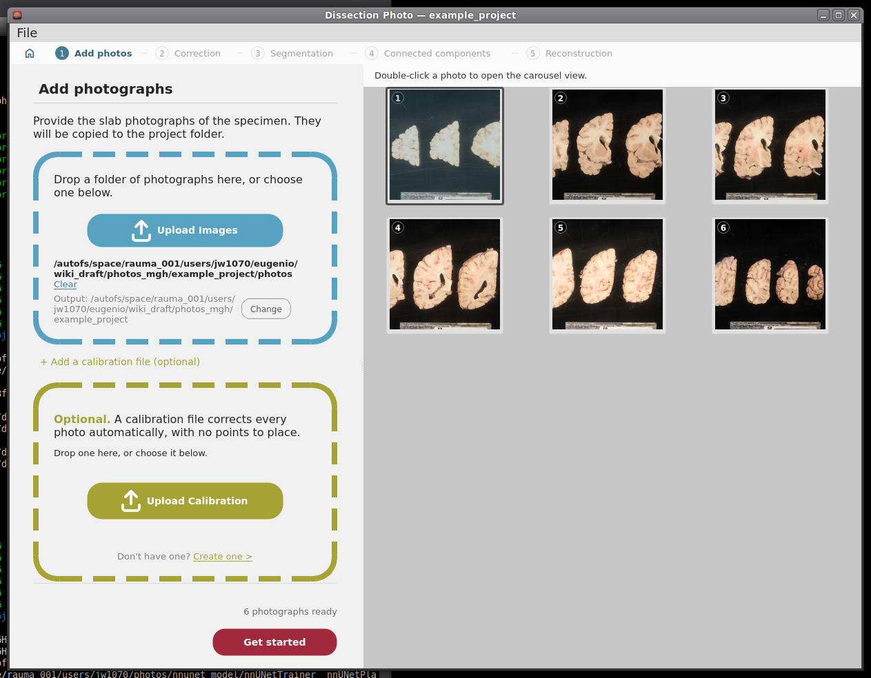
Drag and drop a folder containing dissection photographs, or click Upload Images.
- Select the photographs that should be used for the reconstruction. This can be used to omit repeat photographs, dissection photographs of cerebellar tissue, or gross photographs done prior to slabbing. Double click on any image in the grid for a larger preview.
If you have or would like to create a calibration file to automate pixel correction, click on + Add a calibration file (optional) and follow the steps in Making a Calibration File and then Prospective Correction.
Click Get started.
|
|

Optional: Making a calibration file
This step only needs to be done once, as long as the markers are not moved. For more information on proper usage refer to the Markers for pixel and perspective corrections section of the slab photography page.
On the Add photos menu, click + Add a calibration file (optional) to expand the calibration file box, and click on Create one under the Upload Calibration button.
On the next menu, if you have not printed out the fiducial markers, they can be downloaded for printing by clicking the Download Marker Printout button.
- Next, place markers at a known distance in a rectangle formation on the photography table. Be sure that opposite sides of the rectangle created by the fiducial markers are parallel; inaccurate marker placement can lead to incorrect perspective correction.
- Upload the photograph of the empty dissection table with just the markers present, and enter the width and height of the fiducial box.
- For each of the markers, click its centre and outer circle. Options to zoom, pan, and redo/undo can help fix mistakes and make the best calibration possible.
Click Save Calibration and save your calibration file in an easy-to-access location.
Tip: Because of slight lens distortion, the overlaid labels for the outer circle of the markers might not always align throughout the whole circumference. This is not an issue.

The photograph of the empty table with the four markers, uploaded.
|
|


Step 2: Pixel Correction
This step corrects all photographs to be at the same pixel size. Additionally, it can correct for perspective when using a calibration file, or when doing manual correction in 4-point mode.
Prospective Correction (Using fiducial markers and calibration file)
- Every photo is corrected automatically as soon as Correction opens. The markers are found in each photo separately, so it does not matter if the camera moved between photos.
Check each photo: Original shows the photo as taken, with the marker centres that were found; Corrected shows the result. A green tick in the strip at the bottom marks each corrected photo.
If the markers cannot be found in a photo, the app says which ones. On each of them, click the centres of the four markers on the Original view and click Correct this photo.
Retrospective Correction (Using a spatial reference within the photographs)
Choose how many points you can mark, enter the real distances, and place the points on each photo:
Mode |
You need |
Corrects |
2 Point |
One ruler or other known distance (entered as Ruler width (mm)) |
Pixel size only |
3 Point |
Three corners of a rectangle, e.g. two rulers at right angles |
Pixel size, approximate perspective |
4 Point |
Four corners of a rectangle |
Pixel size and perspective |
Ctrl + left click places a point; once all are placed, Ctrl + click moves the nearest one. Clear points starts again.
Click Correct this photo (Ctrl + W also moves on to the next photo). Place points on the Original view; the Corrected view is for checking.
|
|
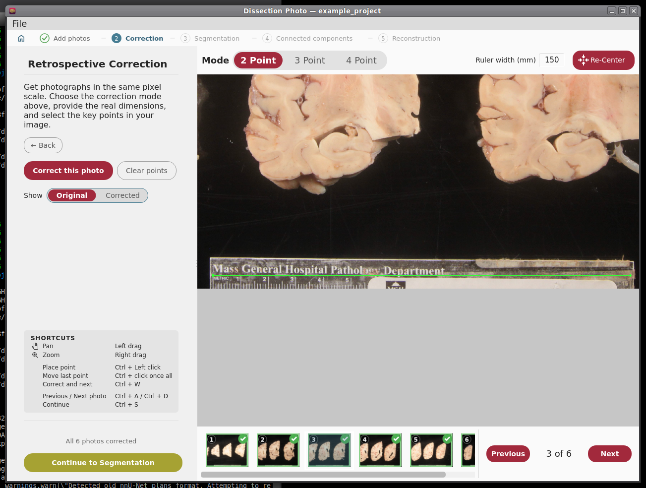
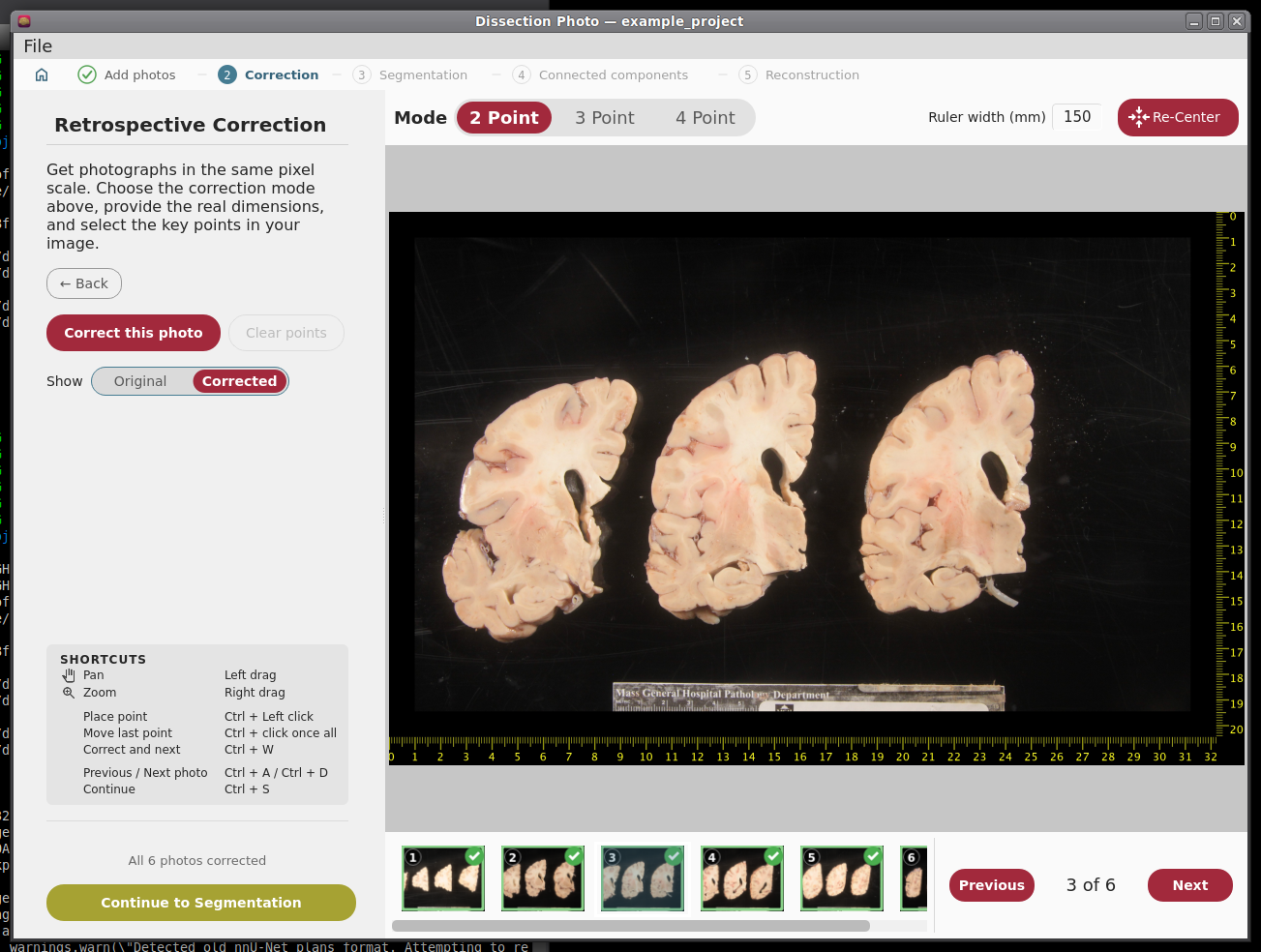
When every photo is corrected, make sure to click Continue to Segmentation.
Step 3: Binary Segmentation
While you were correcting, the app was already finding the tissue in each corrected photo. Here you check each mask and fix it.
|
|
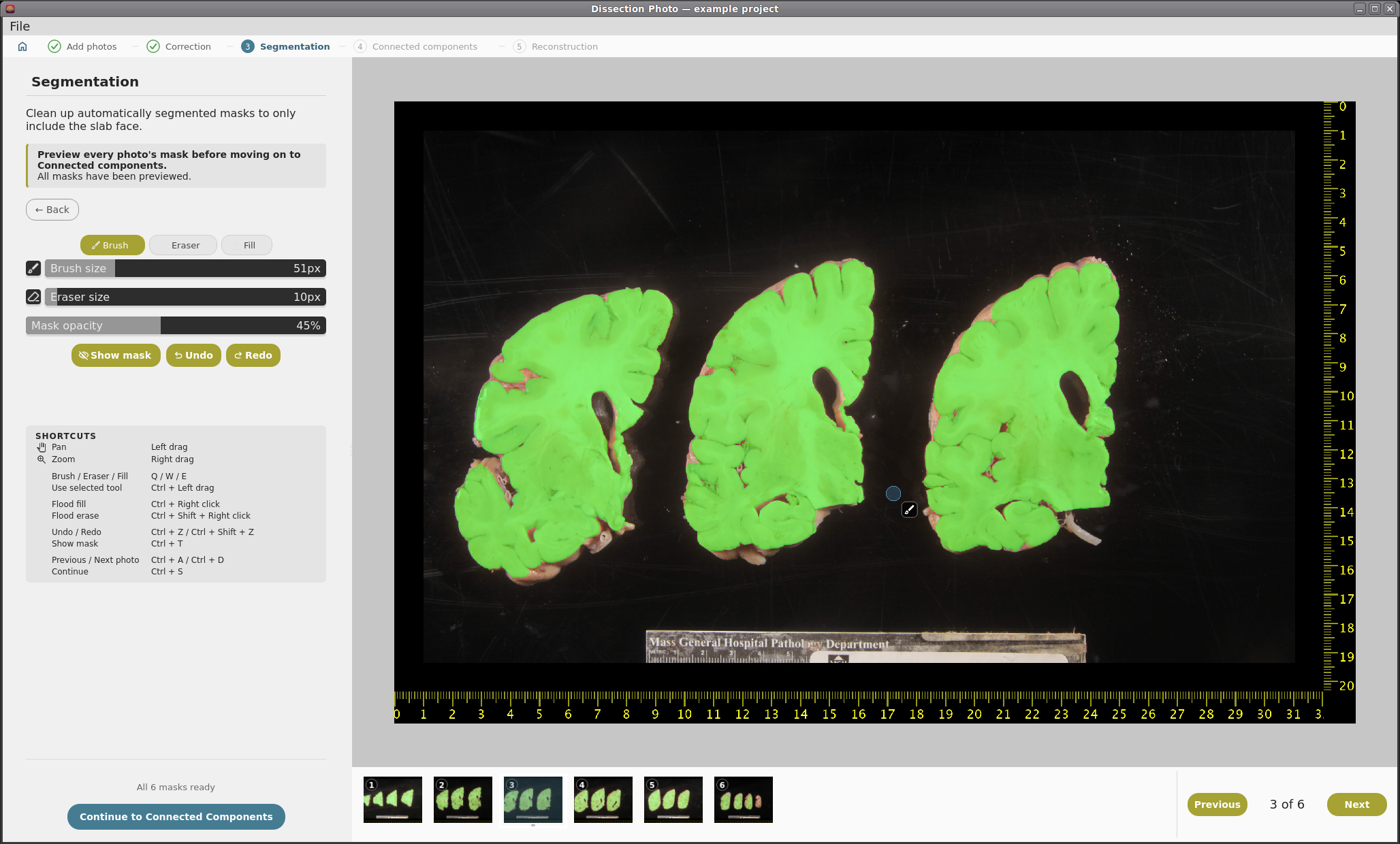
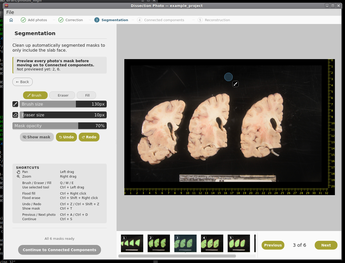
Brush (Q) adds to the mask, Eraser (W) removes from it, and Fill (E) fills an area. Apply the tool with Ctrl + left drag; set the sizes with the sliders.
Mask opacity changes how see-through the mask is; Show mask (Ctrl + T) hides and shows it. Undo and redo with Ctrl + Z and Ctrl + Shift + Z.
- Leave out everything that is not slab tissue: the background, labels, and fragments that do not belong to a slab.
IMPORTANT: the cortical surface should not be part of the masks, so the first slab (if photographed from the anterior side) or the last slab (if photographed from the posterior side) should NOT be included.
You need to look at every photo's mask before Continue to Connected Components becomes available; a note at the top says which ones are left.
Automatic Segmentation Settings
Open them from the gear on the Projects screen. Changes apply the next time photos are segmented.

Automatic segmentation settings.
Setting |
What it does |
Automatic segmentation (On / Off) |
Off: every mask is drawn by hand from scratch. Only turn it off if the automatic segmentation fails on your photos. |
Model folds |
Automatic: 5 folds on a GPU, 1 on the CPU. Five folds are steadier but 4-5x slower. |
Run on |
Automatic uses the GPU if there is one; or choose GPU or CPU. |
Maximum threads |
The most processor threads segmentation may use. If the computer has fewer, it uses all it has. |
Model folder |
The folder of the segmentation model (nnUNetTrainer__nnUNetPlans__2d). |
Step 4: Slab Connected Components
Here you tell the app which pieces of tissue belong to which slab.
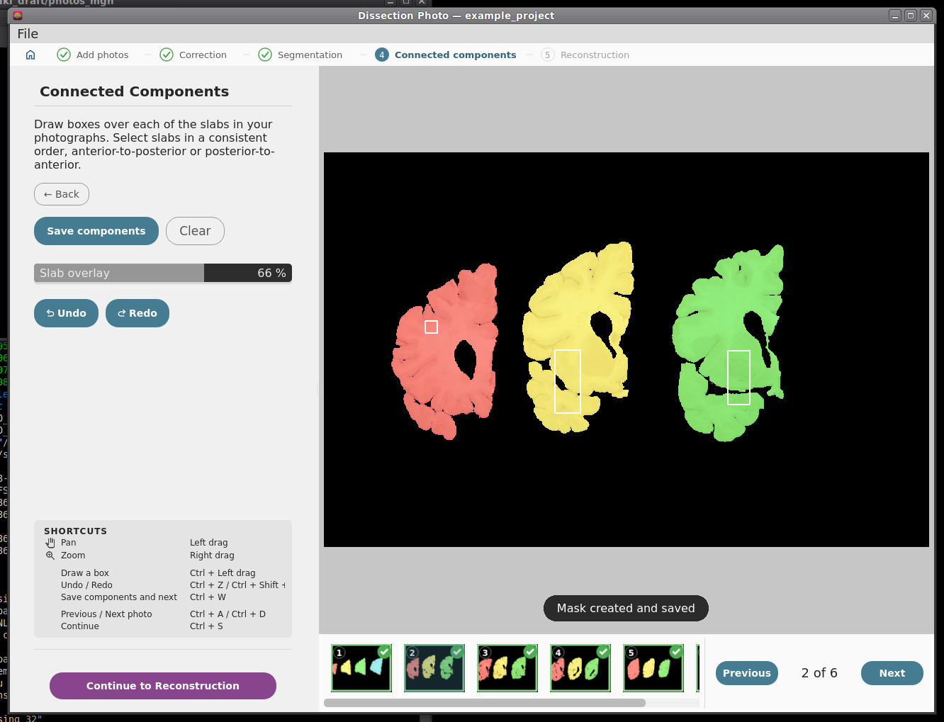
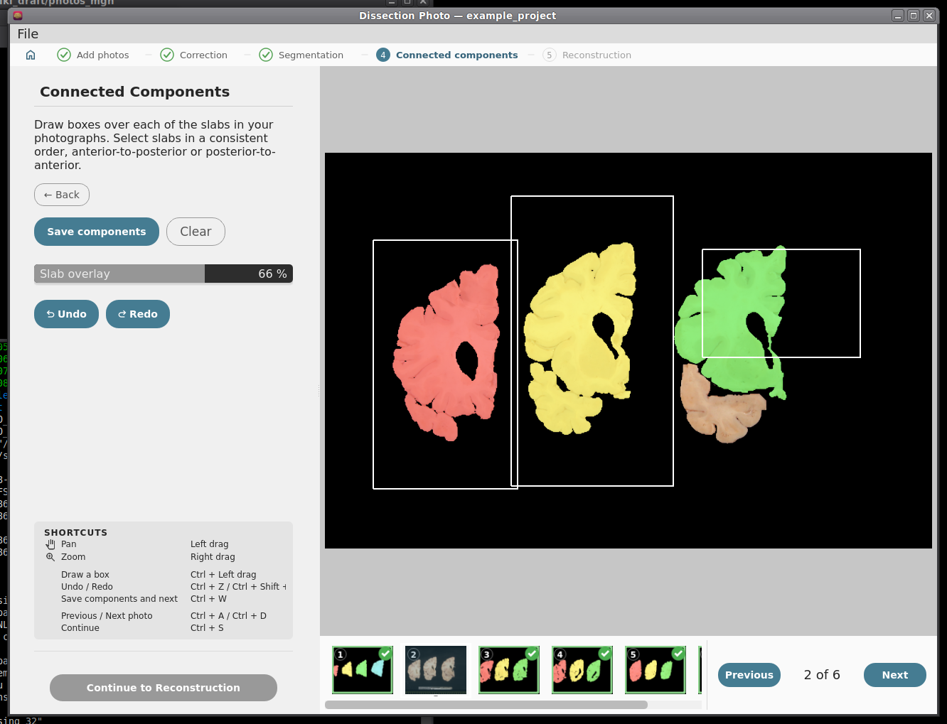
- In each photo, draw a box inside each slab (Ctrl + left drag), always in the same order: anterior to posterior, or posterior to anterior. The slab is colored as soon as its box is drawn.
- Keep boxes small and inside the tissue, and do not let them overlap. If a slab is in several pieces (e.g. a detached temporal lobe), make sure its box touches every piece.
Click Save components (Ctrl + W also moves on to the next photo); moving to another photo saves it too. A green tick marks saved photos. If you change a saved photo, its tick goes away until you save it again.
Undo and redo with Ctrl + Z and Ctrl + Shift + Z. Slab overlay changes how strongly the slabs are colored.
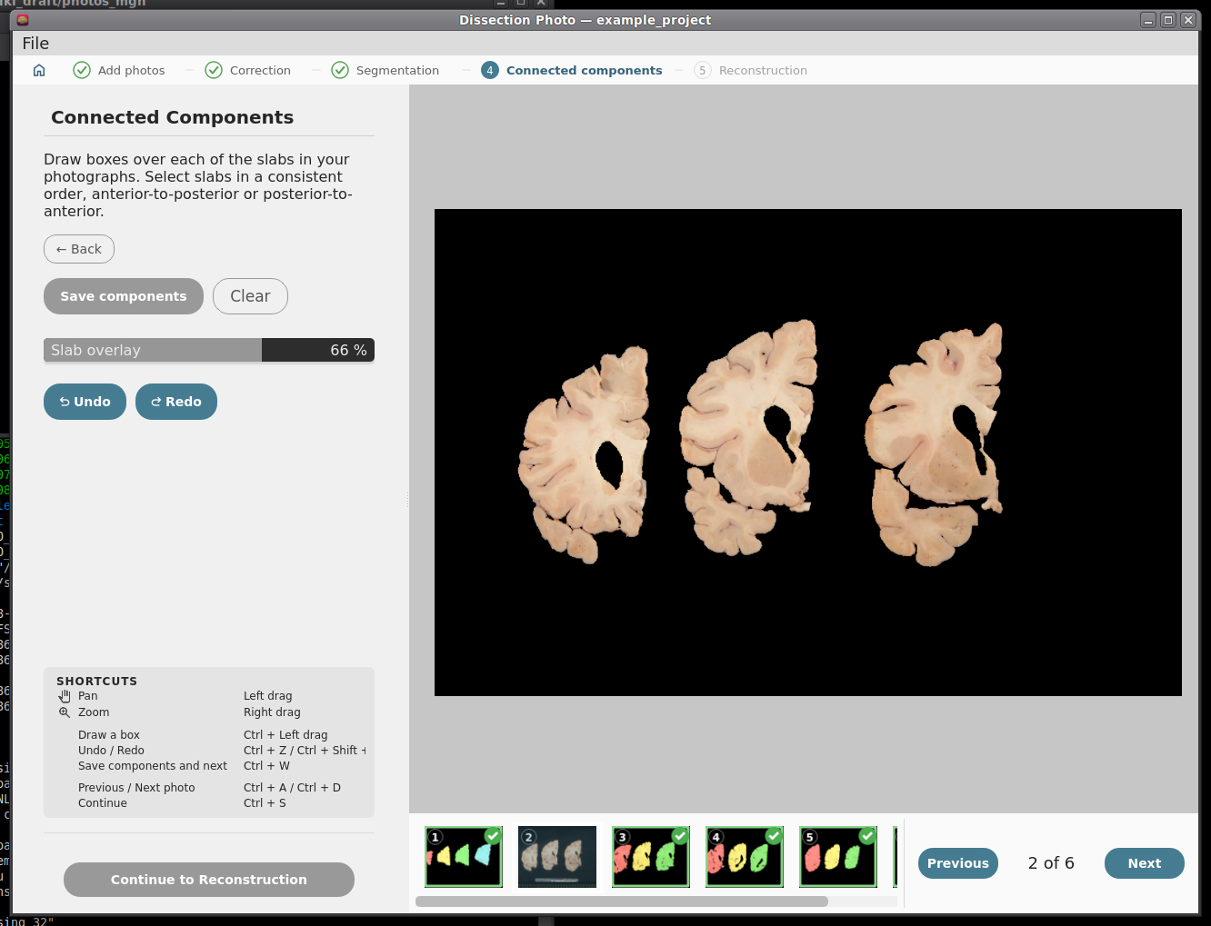
Before any boxes are drawn.
|
|
Step 5: Photo Reconstruction
Please see our separate page on the command mri_3d_photo_recon. The last step runs mri_3d_photo_recon on the images of the project. While the reconstruction is running in the background the user can continue processing images of other cases.
Output folder: the folder inside the project for the results (default recon).
Slabs: the hemisphere, the slab thickness in mm, which face of the slabs was photographed (anterior or posterior), the order the photos were taken in, and whether the tissue is fixed or fresh.
Reference: none (the MNI atlas), a surface mesh (.stl), an MRI scan, or both. See Which reference should I use?
- Optionally: the number of threads, a graphics card, and the advanced settings. Empty expert weights use the command's own defaults, shown in grey.
Click Run Reconstruction.
The command being run is shown on the right (Copy command copies it, for example to run it on another computer), and its output appears in the log below it. The reconstruction keeps running if you switch to another project; the Projects screen shows its progress.

A reconstruction running, with the command and its log.
Part 3: Downstream Tasks
Photo-Synthseg Segmentation
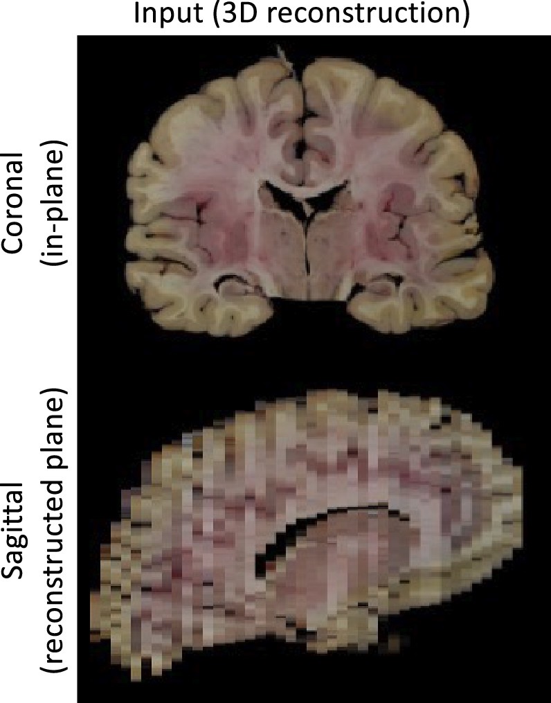
The 3D reconstructed stacks can be segmented with SynthSeg using the flag --photo. Please see the wiki page for SynthSeg for further information.
|
|

Example for running SynthSeg on a Left Hemisphere
mri_synthseg \
--i ./recon/photo_recon.mgz \
--o ./recon/photo_recon_synthseg.mgz \
--photo left \
--parc