Anatomical ROI analysis
This tutorial gives a brief introduction to anatomical ROI analysis which includes working with label files, extracting ROI measures from the anatomical data, group statistics etc.
1. Preparations
1.1. If You're at an Organized Course
If you are taking one of the formally organized courses, everything has been set up for you on the provided laptop. The only thing you will need to do is run the following commands in every new terminal window (aka shell) you open throughout this tutorial. Copy and paste the commands below to get started:
export SUBJECTS_DIR=$TUTORIAL_DATA/buckner_data/tutorial_subjs/group_analysis_tutorial
cd $SUBJECTS_DIR
To copy: Highlight the command in the box above, right click and select copy (or use keyboard shortcut Ctrl+c), then use the middle button of your mouse to click inside the terminal window (this will paste the command). Press enter to run the command. These two commands set the SUBJECTS_DIR variable to the directory where the data is stored and then navigates into this directory. You can now skip ahead to the tutorial (below the gray line).
1.2. If You're not at an Organized Course
If you are NOT taking one of the formally organized courses, then to follow this exercise exactly be sure you've downloaded the tutorial data set before you begin. If you choose not to download the data set you can follow these instructions on your own data, but you will have to substitute your own specific paths and subject names. These are the commands that you need to run before getting started:
<source_freesurfer>
export TUTORIAL_DATA=<path_to_your_tutorial_data>
export SUBJECTS_DIR=$TUTORIAL_DATA/buckner_data/tutorial_subjs/group_analysis_tutorial
cd $SUBJECTS_DIR
If you are not using the tutorial data you should set your SUBJECTS_DIR to the directory in which the recon(s) of the subject(s) you will use for this tutorial are located.
2. Relationship between segmentation, parcellation and LookUp Table (LUT)
In this exercise, you will examine a segmentation, parcellation, and color lookup table to understand how they are related. Open the subject in freeview using the following command and select 'coronal' view at the top menu bar:
freeview -v 004/mri/orig.mgz \
004/mri/aparc+aseg.mgz:colormap=lut:opacity=0.4 \
-f 004/surf/lh.white:annot=aparc.annot
NOTE: The backslash allows you to copy and paste multiple lines of code as one command. We use this throughout the tutorials to display the commands in a more easy-to-read manner, while still allowing you to copy and paste. Whenever you are typing in your own commands, instead of copying and pasting a command written out across multiple lines, a backslash is not necessary.
The above command opens the orig and aparc+aseg segmentation volume (aparc+aseg.mgz) as well as the cortical surface parcellation (aparc.annot) on the white surface in the left hemisphere.
Note that the default parcellation uses the Deskian/Killiany atlas. There is also the option to use the Destrieux atlas parcellation, where the surface is parcellated into more anatomical regions than the Deskian/Killiany atlas.
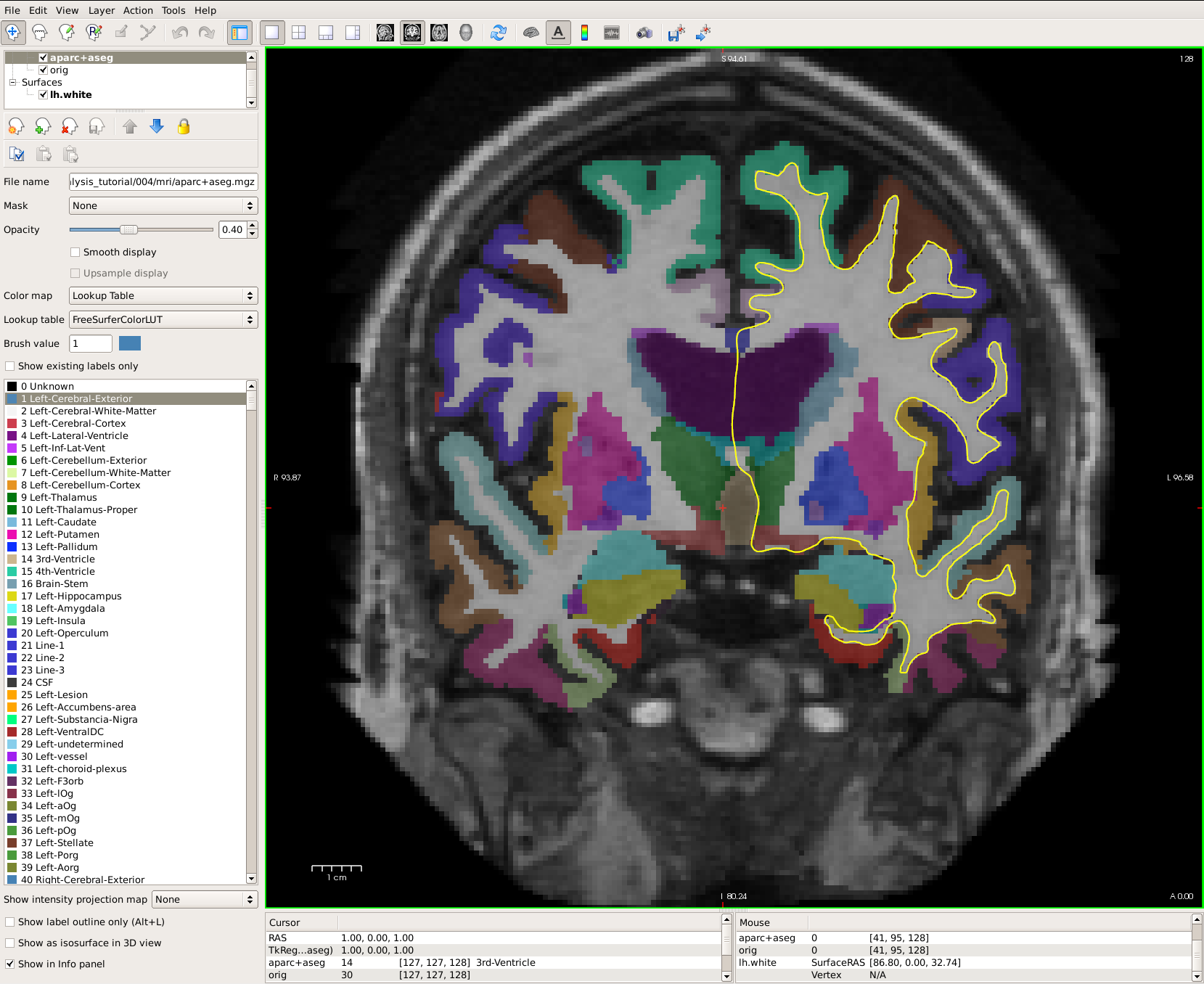
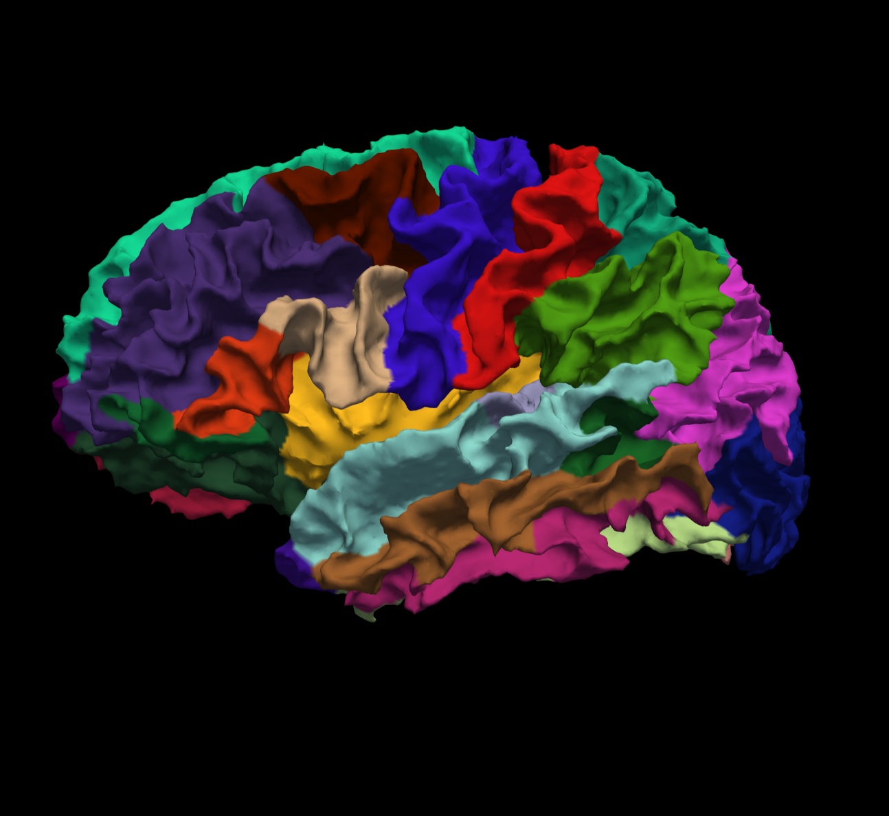
Note: The aparc+aseg.mgz file shows the parcellated cortical ribbon at the same time as the segmented subcortical structures. The "colormap=lut" tells freeview to display the aparc+aseg.mgz file with colors according to the look up table. The aparc+aseg.mgz uses the Desikan-Killiany atlas. To see the Destrieux atlas, you would load fsaverage/mri/aparc.a2009s+aseg.mgz
Run the following command in a new terminal window to display the contents of the LUT (Look Up Table):
less $FREESURFER_HOME/FreeSurferColorLUT.txt
You can hit the 'Page Up' and 'Page Down' buttons on your keyboard to scroll through the text file. Or click here to view the contents of the file. (To exit the less command, hit 'q' on your keyboard.)
Things to do -- Navigating between freeview and the LUT:
- Choose the coronal view and click on a cortical structure in the brain.
- See the structure name next to 'aparc+aseg' in the Cursor section below the main viewing window. For example, it may say ctx-lh-precentral. Notice which hemisphere is specified.
- Look at the number listed immediately after the 'aparc+aseg'. For example, it may say 1024.
- Find that value in the LUT, which you have opened using the command mentioned above.
- Verify that it is the same structure you chose in freeview.
- Do the same with a subcortical structure of your choice.
You can close freeview once you are done. To get out of the less command, type 'q' for quit and hit enter.
3. Label files
To accurately map a manually drawn or pre-existing label of a region of interest to several subjects in your study, you should first register your label to or draw your label on fsaverage (a template to which all subjects run with FreeSurfer have been registered to) and then use the mri_label2label command to map the label to individual subjects. An example of the command you would use is illustrated below using the FreeSurfer-generated lh.BA45.label (Brodmann area 45, part of Broca's area involved in language). Please run:
cd $SUBJECTS_DIR
mri_label2label \
  --srcsubject fsaverage \
  --srclabel fsaverage/label/lh.BA45.label \
  --trgsubject 004 \
  --trglabel 004/label/lh.BA45.label \
  --hemi lh \
  --regmethod surface
For more information about this command, type "mri_label2label --help" inside your terminal.
Important flags:
- --srcsubject (the source subject)
- --srclabel (the input label file from source subject)
- --trgsubject (target subject you are mapping the label to)
- --trglabel (output label file on target subject)
- --regmethod (specify if you want the registration to occur on the surface or in the volume)
Our target subject in this example was 004. You can now view the label on this subject in freeview. First load the subject:
freeview -v 004/mri/orig.mgz
Then on the menu bar click File > Load ROI  choose lh.BA45.label and hit 'Open'. The label is visible in coronal slice 153. To jump to that slice, double click on the coordinates [127,127,128] next to where it says 'orig' in the Cursor window pane. The last number is the slice number. Change it to 153 and hit enter.
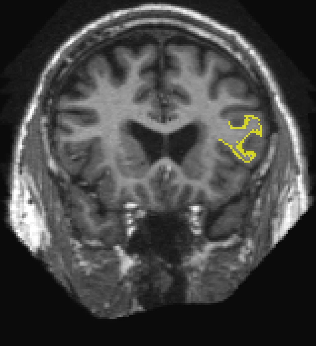
To view the label on the surface, first load the the subject's inflated surface in freeview (in another terminal window) using the command below. At the top menu bar, select the 3D view.
freeview -f 004/surf/lh.inflated
On the left menu, click on the drop down menu next to 'Curvature' and select 'Off'. Next to 'Label', select 'Load'. In the window that pops up, navigate to the label directory if it is not already in it and select lh.BA45.label. Hit 'OK'. The label loaded on the inflated surface will look like this:
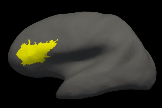
Note: If you want to use a pre-existing label and register it to fsaverage, be aware that this might involve two instances of resampling and the results might not be as accurate as they would be if you drew the label on fsaverage. Please contact the FreeSurfer team to get more details on this process if you have any concerns.
You can close freeview once you are done.
3.1. Creating a Single Label
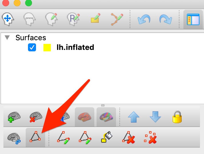
In FS version 7.1.1 If you just need one label you can create a label instead of annotations. You can click “Path/Custom Fill” icon on the left panel, draw a closed path and use custom fill tool to draw a label. Just like in TkSurfer if you have used it before.
4. Individual Stats files
During the FreeSurfer processing stream, via the recon-all script, some statistical output files are generated. They are kept in each subjects' stats/ subdirectory and are generated for the subcortical segmentation (aseg) and the cortical parcellation (aparc). These tables include information on each labeled region for the individual subject. You can view these output files via the terminal or a text editor.
4.1. aseg.stats
The statistical output from the subcortical segmentation, called aseg.stats, is a regular text file and will contain the volumes of specific structures. For example, you can obtain information such as the volume of left hippocampus and its mean intensity from this file.
cd $SUBJECTS_DIR/004/stats
less aseg.stats
At the head of the text file there will be information about the command that was run, the version used, the user who ran it and a time stamp. Following this there is information about the volume of the entire brain.
The next section of this file defines the column headers, field name, and units for the rest of the table. We can expect to see the Segmentation Id, Number of Voxels, Volume, Structure Name, Intensity normMean, Intensity normStdDev, Intensity normMin, Intensity normMax, and Intensity normRange for each entry in the table. The "norm" stats are extracted for each segmented structure from $SUBJECTS_DIR/004/mri/norm.mgz.
The remainder of the table shows this information for all the structures that are labeled in the aseg. (Remember, press 'q' if you want to quit the 'less' command).
# Title Segmentation Statistics
#
# generating_program mri_segstats
# cvs_version $Id: mri_segstats.c,v 1.75.2.2 2011/04/27 22:18:58 nicks Exp $
# cmdline mri_segstats --seg mri/aseg.mgz --sum stats/aseg.stats --pv mri/norm.mgz --empty --excludeid 0 --excl-ctxgmwm --supratent --subcortgray --in mri/norm.mgz --in-intensity-name norm --in-intensity-units MR --etiv --surf-wm-vol --surf-ctx-vol --totalgray --ctab /usr/local/freesurfer/stable5_1_0/ASegStatsLUT.txt --subject 004
# sysname  Linux
# hostname compute-0-36.local
# machine  x86_64
# user     khoa
# anatomy_type volume
#
# SUBJECTS_DIR /autofs/cluster/freesurfer/test/subjects/x86_64/buckner_data/group_study_fs5.1.0
# subjectname 004
# Measure lhCortex, lhCortexVol, Left hemisphere cortical gray matter volume, 243583.395631, mm^3
# Measure rhCortex, rhCortexVol, Right hemisphere cortical gray matter volume, 245552.725775, mm^3
# Measure Cortex, CortexVol, Total cortical gray matter volume, 489136.121407, mm^3
# Measure lhCorticalWhiteMatter, lhCorticalWhiteMatterVol, Left hemisphere cortical white matter volume, 257212.437500, mm^3
# Measure rhCorticalWhiteMatter, rhCorticalWhiteMatterVol, Right hemisphere cortical white matter volume, 254883.390625, mm^3
# Measure CorticalWhiteMatter, CorticalWhiteMatterVol, Total cortical white matter volume, 512095.828125, mm^3
# Measure SubCortGray, SubCortGrayVol, Subcortical gray matter volume, 180840.000000, mm^3
# Measure TotalGray, TotalGrayVol, Total gray matter volume, 669976.121407, mm^3
# Measure SupraTentorial, SupraTentorialVol, Supratentorial volume, 1181347.254146, mm^3
# Measure IntraCranialVol, ICV, Intracranial Volume, 1792908.998979, mm^3
# SegVolFile mri/aseg.mgz
# SegVolFileTimeStamp  2011/05/18 20:50:12
# ColorTable /usr/local/freesurfer/stable5_1_0/ASegStatsLUT.txt
# ColorTableTimeStamp 2011/05/14 14:56:11
# InVolFile  mri/norm.mgz
# InVolFileTimeStamp  2011/05/18 13:09:34
# InVolFrame 0
# PVVolFile  mri/norm.mgz
# PVVolFileTimeStamp  2011/05/18 13:09:34
# Excluding Cortical Gray and White Matter
# ExcludeSegId 0 2 3 41 42
# VoxelVolume_mm3 1
# TableCol  1 ColHeader Index
# TableCol  1 FieldName Index
# TableCol  1 Units     NA
# TableCol  2 ColHeader SegId
# TableCol  2 FieldName Segmentation Id
# TableCol  2 Units     NA
# TableCol  3 ColHeader NVoxels
# TableCol  3 FieldName Number of Voxels
# TableCol  3 Units     unitless
# TableCol  4 ColHeader Volume_mm3
# TableCol  4 FieldName Volume
# TableCol  4 Units     mm^3
# TableCol  5 ColHeader StructName
# TableCol  5 FieldName Structure Name
# TableCol  5 Units     NA
# TableCol  6 ColHeader normMean
# TableCol  6 FieldName Intensity normMean
# TableCol  6 Units     MR
# TableCol  7 ColHeader normStdDev
# TableCol  7 FieldName Itensity normStdDev
# TableCol  7 Units     MR
# TableCol  8 ColHeader normMin
# TableCol  8 FieldName Intensity normMin
# TableCol  8 Units     MR
# TableCol  9 ColHeader normMax
# TableCol  9 FieldName Intensity normMax
# TableCol  9 Units     MR
# TableCol 10 ColHeader normRange
# TableCol 10 FieldName Intensity normRange
# TableCol 10 Units     MR
# NRows 45
# NTableCols 10
# ColHeaders  Index SegId NVoxels Volume_mm3 StructName normMean normStdDev normMin normMax normRange
  1   4     31490    31490.0  Left-Lateral-Ventricle            13.5672    11.0434     0.0000    79.0000    79.0000
  2   5      1416     1416.0  Left-Inf-Lat-Vent                 32.9812    14.4618     4.0000    87.0000    83.0000
  3   7     13623    13623.0  Left-Cerebellum-White-Matter      88.0573     8.7477    41.0000   123.0000    82.0000
  4   8     46105    46105.0  Left-Cerebellum-Cortex            58.5936     9.9359    16.0000   100.0000    84.0000
  5  10      6951     6951.0  Left-Thalamus-Proper              83.1834    11.8098    16.0000   121.0000   105.0000
  6  11      5942     5942.0  Left-Caudate                      67.7429    12.2442    22.0000    99.0000    77.0000
  7  12      8828     8828.0  Left-Putamen                      74.2015    10.0100    21.0000   107.0000    86.0000
-
-
4.2. aparc.stats
The statistical output from the cortical parcellation, called lh.aparc.stats and rh.aparc.stats, is a regular text file and will contain the thickness of specific structures. For example, you can obtain information such as, how big is left superior temporal gyrus and its average thickness from this file.
cd $SUBJECTS_DIR/004/stats
less lh.aparc.stats
This file takes the same format as the aseg.stats. The measures at the top show the number of vertices in the cortex (NumVert) and the surface area of the cortex (SurfArea). This part of the file also tells us that the lh.aparc.annot is being used as the annotation file (AnnotationFile ../label/lh.aparc.annot).
The next section of this file defines the column headers, field name, and units for the rest of the table. We can expect to see the Structure Name, Number of Vertices, Surface Area, Gray Matter Volume, Average Thickness, Thickness StDev, Integrated Rectified Mean Curvature, Integrated Rectified Gaussian Curvature, Folding Index and Intrinsic Curvature Index for each entry in the table.
The remainder of the table shows this information for all the structures that are labeled in the aparc. (Again 'q' will exit 'less').
# Table of FreeSurfer cortical parcellation anatomical statistics
#
# CreationTime 2011/10/21-15:36:36-GMT
# generating_program mris_anatomical_stats
# cvs_version $Id: mris_anatomical_stats.c,v 1.72 2011/03/02 00:04:26 nicks Exp $
# mrisurf.c-cvs_version $Id: mrisurf.c,v 1.693.2.2 2011/04/27 19:21:05 nicks Exp $
# cmdline mris_anatomical_stats -mgz -cortex ../label/lh.cortex.label -f ../stats/lh.aparc.stats -b -a ../label/lh.aparc.annot -c ../label/aparc.annot.ctab 004 lh white
# sysname  Linux
# hostname compute-0-36.local
# machine  x86_64
# user     khoa
#
# SUBJECTS_DIR /autofs/cluster/freesurfer/test/subjects/x86_64/buckner_data/group_study_fs5.1.0
# anatomy_type surface
# subjectname 004
# hemi lh
# AnnotationFile ../label/lh.aparc.annot
# AnnotationFileTimeStamp 2011/10/21 11:22:04
# Measure Cortex, NumVert, Number of Vertices, 139655, unitless
# Measure Cortex, WhiteSurfArea, White Surface Total Area, 94794.7, mm^2
# Measure Cortex, MeanThickness, Mean Thickness, 2.31382, mm
# NTableCols 10
# TableCol  1 ColHeader StructName
# TableCol  1 FieldName Structure Name
# TableCol  1 Units     NA
# TableCol  2 ColHeader NumVert
# TableCol  2 FieldName Number of Vertices
# TableCol  2 Units     unitless
# TableCol  3 ColHeader SurfArea
# TableCol  3 FieldName Surface Area
# TableCol  3 Units     mm^2
# TableCol  4 ColHeader GrayVol
# TableCol  4 FieldName Gray Matter Volume
# TableCol  4 Units     mm^3
# TableCol  5 ColHeader ThickAvg
# TableCol  5 FieldName Average Thickness
# TableCol  5 Units     mm
# TableCol  6 ColHeader ThickStd
# TableCol  6 FieldName Thickness StdDev
# TableCol  6 Units     mm
# TableCol  7 ColHeader MeanCurv
# TableCol  7 FieldName Integrated Rectified Mean Curvature
# TableCol  7 Units     mm^-1
# TableCol  8 ColHeader GausCurv
# TableCol  8 FieldName Integrated Rectified Gaussian Curvature
# TableCol  8 Units     mm^-2
# TableCol  9 ColHeader  FoldInd
# TableCol  9 FieldName  Folding Index
# TableCol  9 Units      unitless
# TableCol 10 ColHeader CurvInd
# TableCol 10 FieldName Intrinsic Curvature Index
# TableCol 10 Units     unitless
# ColHeaders StructName NumVert SurfArea GrayVol ThickAvg ThickStd MeanCurv GausCurv FoldInd CurvInd
bankssts                                 1519   1044   2415  2.257 0.498     0.137     0.046       19     2.9
caudalanteriorcingulate                  1296    855   2535  2.713 0.741     0.163     0.074       29     3.5
caudalmiddlefrontal                      3322   2216   6445  2.578 0.561     0.142     0.056       42     7.7
cuneus                                   2467   1593   2996  1.742 0.393     0.173     0.081       49     8.0
entorhinal                                558    408   1936  3.268 0.935     0.138     0.052        6     1.2
-
-
-
5. Group stats files
This section will run you through using the stats directory of the subjects to perform group stats of certain structures that may be of interest to your study. The following commands will help you combine the data of the subjects you are analyzing into one table that will be easily read into a spreadsheet program. We have considered 6 subjects as examples (004, 021, 040, 067, 080, 092) in the following sections. Set your SUBJECTS_DIR to the path where you have your subjects to be analyzed.
export SUBJECTS_DIR=$TUTORIAL_DATA/buckner_data/tutorial_subjs/group_analysis_tutorial
cd $SUBJECTS_DIR
5.1. Table of segmentation volumes
This section explains how to create a table of segmentation volumes using the 6 subjects mentioned above.
asegstats2table --subjects 004 021 040 067 080 092 \
  --segno 11 17 18 \
  --tablefile aseg.vol.table
where 11, 17 and 18 correspond to the segmentation label of left caudate, left hippocampus and left amygdala respectively. (You can create a table with all of the labels, not just these three, by omitting the --segno part.) Click here if you would like to view the list of labels and their corresponding ID numbers again.
The file aseg.vol.table is your output - a text file consisting of the subjects mentioned in the command above and the values for the structures requested along with the measures in the header. The information in this text file is formatted so it can be easily imported into a spreadsheet program (often used as input for many statistical analysis programs). If you do the ls command, you should see that the text file aseg.vol.table has been created. To see what the file looks like, do:
less aseg.vol.table
(press 'q' to exit). To see what the file looks like, you can open it with gedit or any other text editing or spreadsheet application:
gedit aseg.vol.table
Note: Mac users should run
open -e aseg.vol.table
In the table, the first cell is volume indicating that the measure is a volume in mm3 for all of the cells to the right. The subject IDs can be found below volume (seen as 4, 21, 40, 67, 80, 92). You'll notice that in the examples we've considered here for asegstats2table, each subject is a 3 digit number (004, 021 etc).
5.2. Table of segmentation mean intensities
The purpose of this section is to demonstrate how you can change what measure you collect for your spreadsheet from volume to mean intensity using the asegstats2table command.
asegstats2table \
  --subjects 004 021 040 067 080 092 \
  --segno 11 17 18 \
  --meas mean \
  --tablefile aseg.mean-intensity.table
You can load the table into a spreadsheet as explained in the previous section or view aseg.mean-intensity.table with a text editor, like gedit.
5.3. Table of white matter parcellation volumes
The purpose of this section is to show how you can change which segmentation atlas you get stats from (and thus which structures):
asegstats2table \
  --subjects 004 021 040 067 080 092 \
  --segno 3007 3021 3022 4022 \
  --stats wmparc.stats \
  --tablefile wmparc.vol.table
This prints out stats on the white matter parcellation.
5.4. Table of the surface area of each cortical parcellation in the Desikan atlas
This section demonstrates how to create a table of the surface area of each cortical parcellation in the Desikan atlas (surface area is the default measure).
aparcstats2table --hemi lh \
  --subjects 004 021 040 067 080 092 \
  --tablefile lh.aparc.area.table
Feel free to take a look at those results.
5.5. Table of the average thickness of each cortical parcellation in the Destrieux atlas
The purpose of this section is to show how to change the summary measure (in this case, to thickness) and the parcellation atlas (to Destrieux's atlas).
aparcstats2table --hemi lh \
  --subjects 004 021 040 067 080 092 \
  --meas thickness \
  --parc aparc.a2009s \
  --tablefile lh.aparc.a2009.thickness.table
You can now load the resulting table into a spreadsheet.
Remember, for more information on individual flags or how to use these commands, you can run:
aparcstats2table --help

asegstats2table --help
