Group Analysis command lines
To follow this exercise exactly be sure you've downloaded the tutorial data set before you begin. If you choose not to download the data set you can follow these instructions on your own data, but you will have to substitute your own specific paths and subject names.
In order to compute the contrasts you will first need to change to the tutorial data directory and setup SUBJECTS_DIR:
cd $TUTORIAL_DATA/buckner_data/tutorial_subjs/group_analysis_tutorial
setenv SUBJECTS_DIR ${PWD}
Change into the directory you ran the estimation step in, most likely called 'stats':
cd stats
Upon successful completion of the make_average_subject command you should have an average subject in your SUBJECTS_DIR. After successfully completing Exercise A. and Exercise B. you should have an FSGD file called my_gender_age_fsgd.txt and a contrast file called age.mat, both in your SUBJECTS_DIR/stats directory. Confirm that those files exist:
ls my_gender_age_fsgd.txt age.mat
If my_gender_age_fsgd.txt does not exist, complete Exercise A. If age.mat does not exist, complete Exercise B., or just create a file called age.mat containing this line:
0 0 1
The following are sample commands, that can be used with the data, to complete a group analysis:
# For the left hemisphere

mris_preproc --fsgd my_gender_age_fsgd.txt \
  --target average \
  --hemi lh \
  --meas thickness \
  --out lh.my_gender_age.thickness.mgh
Once this completes you should see the file lh.my_gender_age.thickness.mgh. The next step, the smoothing step, will use this as input:
mri_surf2surf --hemi lh \
  --s average \
  --sval lh.my_gender_age.thickness.mgh \
  --fwhm 10 \
  --tval lh.my_gender_age.thickness.10.mgh
Once this is complete you should see the file lh.my_gender_age.thickness.10.mgh. The next step will test the hypothesis you've set up using your contrast vector:
mri_glmfit --y lh.my_gender_age.thickness.10.mgh \
  --fsgd my_gender_age_fsgd.txt doss \
  --glmdir lh.my_gender_age.glmdir \
  --pca \
  --surf average lh \
  --C age.mat
You should have two new directories in $TUTORIAL_DATA/buckner_data/tutorial_subjs/group_analysis_tutorial/stats - lh.my_gender_age.glmdir and rh.my_gender_age.glmdir. If you do:
ls lh.my_gender_age.glmdir
you should see this:
age/     beta.mgh  fsgd.X.mat      pca-eres/  rvar.mgh  y.fsgd
ar1.mgh  eres.mgh  mri_glmfit.log  rstd.mgh   Xg.dat
and if you do:
ls lh.my_gender_age.glmdir/age
you should see this:
C.dat F.mgh gamma.mgh maxvox.dat sig.mgh
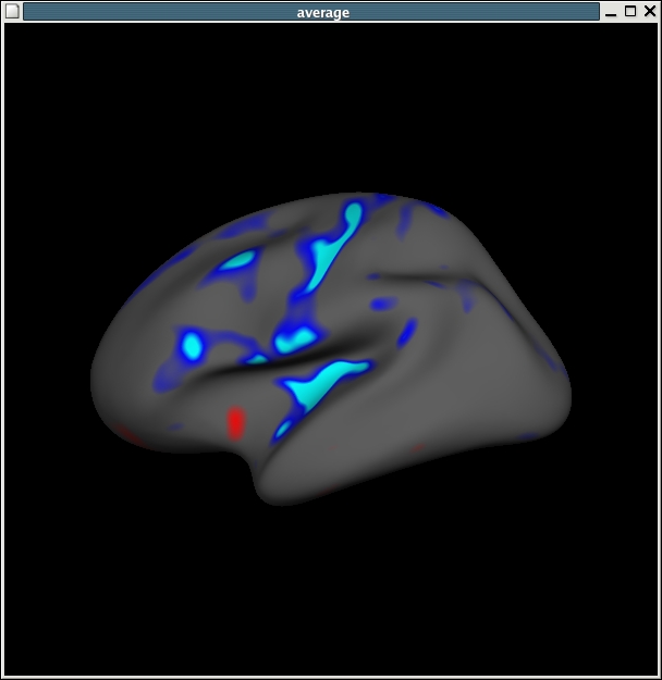
You can view your results by opening the average subject in tksurfer:
tksurfer average lh inflated
and loading in your overlay, File -> Load Overlay and browse to stats/lh.my_gender_age.glmdir/age/sig.mgh.
It should look like this: 
If you would like to also view the scatter plots associated with this you can do so by File -> Load Group Descriptor File and browse to stats/lh.my_gender_age.glmdir/y.fsgd. Once that file is loaded, a window titled 'Thickness' will appear. Once that appears, then click on any point on the surface, and the thickness data for that surface vertex will appear in the Thickness plot window. The surface areas in blue indicating cortical thinning with age, as shown in the plot.
The commands are the same for the right hemisphere, replacing every lh with an rh.
