Clusterwise Correction for Multiple Comparisons
Note: The method used is based on: Smoothing and cluster thresholding for cortical surface-based group analysis of fMRI data. Hagler DJ Jr, Saygin AP, Sereno MI. NeuroImage (2006).
Note: This is the old method for multiple comparisons, for the new tutorial [[
Preparations
If You're at an Organized Course
If you are taking one of the formally organized courses, everything has been set up for you on the provided laptop. The only thing you will need to do is run the following commands in every new terminal window (aka shell) you open throughout this tutorial. Copy and paste the commands below to get started:
export SUBJECTS_DIR=$TUTORIAL_DATA/buckner_data/tutorial_subjs/group_analysis_tutorial
cd $SUBJECTS_DIR/glm
To copy: Highlight the command in the box above, right click and select copy (or use keyboard shortcut Ctrl+c), then use the middle button of your mouse to click inside the terminal window to paste the command (or use keyboard shortcut Ctrl+Shift+v). Press enter to run the command.
These two commands set the SUBJECTS_DIR variable to the directory where the data is stored and then navigates into the sub-directory you'll be working in. You can now skip ahead to the tutorial (below the gray line).
If You're Not at an Organized Course
If you are NOT taking one of the formally organized courses, then to follow this exercise exactly be sure you've downloaded the tutorial data set before you begin. If you choose not to download the data set, you can follow these instructions on your own data, but you will have to substitute your own specific paths and subject names. These are the commands that you need to run before getting started:
## bash
<source_freesurfer>
export TUTORIAL_DATA=<path_to_your_tutorial_data>
export SUBJECTS_DIR=$TUTORIAL_DATA/buckner_data/tutorial_subjs/group_analysis_tutorial
cd $SUBJECTS_DIR/glm
## tcsh
source $FREESURFER_HOME/SetUpFreeSurfer.csh
setenv TUTORIAL_DATA <path_to_your_tutorial_data>
setenv SUBJECTS_DIR $TUTORIAL_DATA/buckner_data/tutorial_subjs/group_analysis_tutorial
cd $SUBJECTS_DIR/glm
Information on how to source FreeSurfer is located here.
If you are not using the tutorial data, you should set your SUBJECTS_DIR to the directory in which the recon(s) of the subject(s) you will use for this tutorial are located.
Introduction
To perform a cluster-wise correction for multiple comparisons, we will run a simulation. The simulation is a way to get a measure of the distribution of the maximum cluster size under the null hypothesis. This is done by iterating over the following steps:
- Synthesize a z map.
- Smooth z map (using residual FWHM).
- Threshold z map (indicate the level and sign of threshold).
- Find clusters in thresholded map.
- Record area of maximum cluster.
Repeat over desired number of iterations (usually > 5,000).
In FreeSurfer, this information is stored in a simple text file called a CSD (Cluster Simulation Data) file.
Once we have the distribution of the maximum cluster size, we correct for multiple comparisons by:
- Going back to the original data.
- Thresholding using same level and sign.
- Finding clusters in thresholded map.
- For each cluster, p = probability of seeing a maximum cluster that size or larger during simulation.
Run the simulation
All these steps are performed with the command mri_glmfit-sim:
mri_glmfit-sim \
  --glmdir lh.gender_age.glmdir \
  --cache 4.0 neg \
  --cwp  0.05\
  --2spaces
Notes:
- Specify the same GLM directory (--glmdir).
- Use precomputed Z Monte Carlo simulation (--cache).
Vertex-wise/cluster-forming threshold of 4 (p < .0001).
- Specify the sign ("neg" for negative, "pos" for positive, or "abs" for absolute/unsigned).
--cwp 0.05 : Keep clusters that have cluster-wise p-values < 0.05. To see all clusters, set to .999.
- --2spaces : adjust p-values for two hemispheres (this assumes you will eventually look at the right hemisphere too).
- You can also generate your own precomputed data, but you only need to do this if you have a different average subject or you are not looking over all of the cortex.
- You can also use a permutation simulation instead of Z Monte Carlo. Run mri_glmfit-sim --help to get more information.
View the Corrected Results
In the contrast subdirectory, you will see several new files by running:
ls lh.gender_age.glmdir/lh-Avg-thickness-age-Cor
You will see the following new files:
cache.th40.neg.pdf.dat -- probability distribution function of clusterwise correction
cache.th40.neg.sig.cluster.mgh -- cluster-wise corrected map (overlay)
cache.th40.neg.sig.cluster.summary -- summary of clusters (text)
cache.th40.neg.sig.masked.mgh -- uncorrected sig values masked by the clusters that survive correction
cache.th40.neg.sig.ocn.annot -- output cluster number (annotation of clusters)
cache.th40.neg.sig.ocn.mgh -- output cluster number (segmentation showing where each numbered cluster is)
cache.th40.neg.sig.voxel.max.dat -- maximum voxel-wise significance
cache.th40.neg.sig.voxel.mgh -- voxel-wise map corrected for multiple comparisons at a voxel (rather than cluster) level
cache.th40.neg.sig.y.ocn.dat -- the average value of each subject in each cluster
First, look at the cluster summary (or click here):
less lh.gender_age.glmdir/lh-Avg-thickness-age-Cor/cache.th40.neg.sig.cluster.summary
You can hit the 'Page Up' and 'Page Down' buttons or the 'Up' and 'Down' arrow keys to see the rest of the file. (To exit the less command, hit the 'q' button.) Notes:
- This is a list of all the clusters that were found (19 of them).
- The CWP column is the cluster-wise probability (the number you are interested in). It is a simple p (ie, NOT -log10(p)).
- For example, cluster number 1 has a CWP of p=.0002.
Load the cluster annotation in freeview:
freeview -f $SUBJECTS_DIR/fsaverage/surf/lh.inflated:overlay=lh.gender_age.glmdir/lh-Avg-thickness-age-Cor/cache.th40.neg.sig.cluster.mgh:overlay_threshold=2,5:annot=lh.gender_age.glmdir/lh-Avg-thickness-age-Cor/cache.th40.neg.sig.ocn.annot -viewport 3d -layout 1
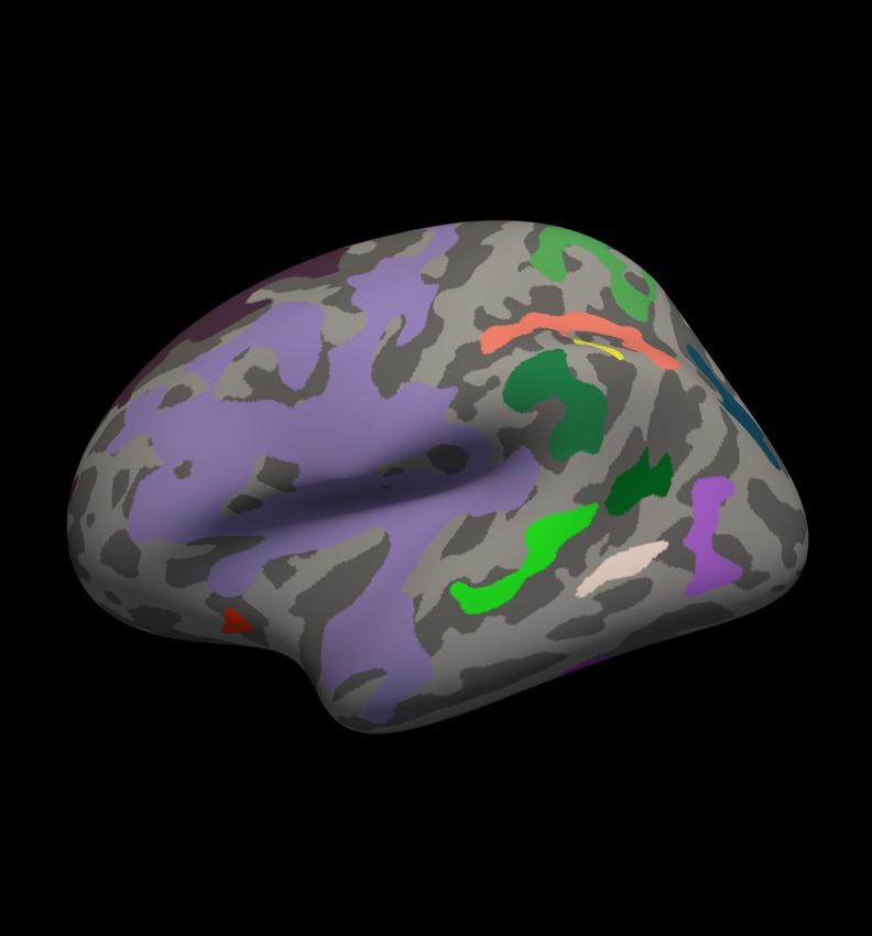
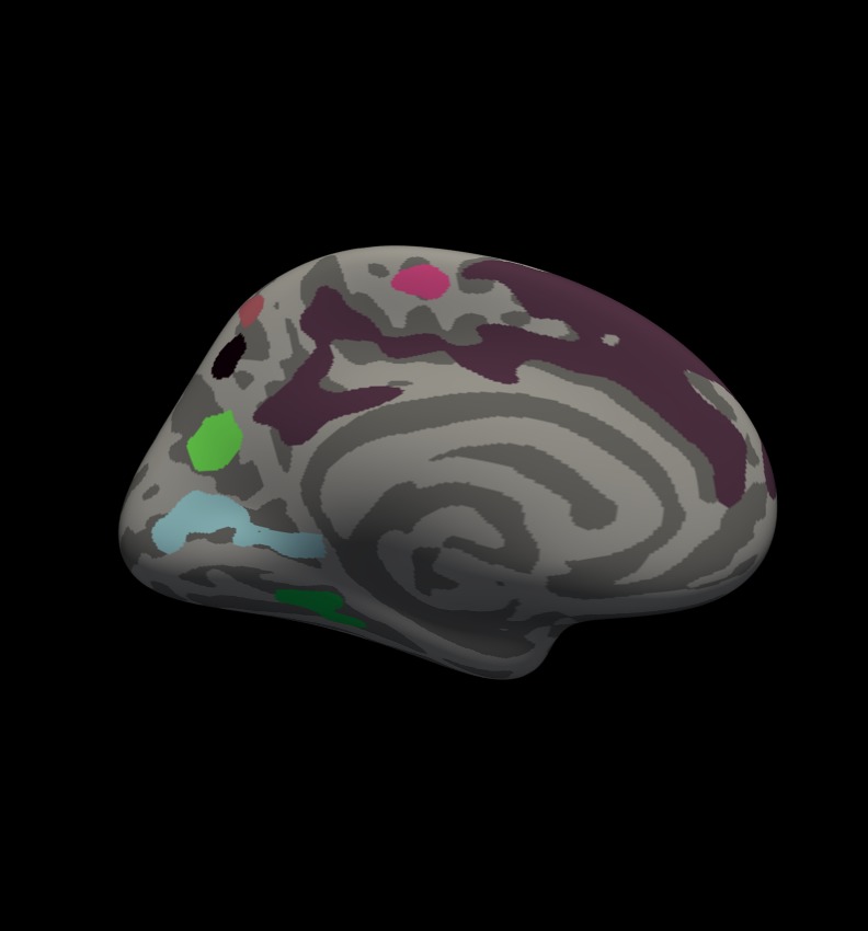
You should see clusters similar in shape to those pictured in the snapshots below. The color values associated with each cluster are arbitrary and may be different:


Notes:
- These are all clusters, regardless of significance.
- When you click on a cluster, the label will tell you the cluster number (eg, cluster-016).
Things to do:
- Find and click on cluster 1 (the largest cluster). It has a value of -3.69899 since this is log10(.0002). The -3.69899 is because the correlation is negative.
Find and click on cluster 18 (on the lateral side of the brain). Its value is -1.70115 because this is log10(0.01990). Note that if you turn off the annotation, the cluster 17 is not visible because its significance is worse than the threshold we set (-fthresh 2, p < .01).
- All vertices within a cluster are the same value (the p-value of the cluster).
You can change the cluster-wise threshold by first clicking on "Show outline only" underneath the Annotation drop down menu. Then click on Configure (underneath "Overlay"), and set the Min value to your desired level. Alternatively, you can drag the red flag to adjust the cluster-wise threshold. As you do this, clusters will appear or disappear from the surface. (If your cursor is in the Min text box, the red flag won't move. Click on another text box to be able to move the flag.)
Study Questions
Where is the information from the simulation stored? Answer
What are the steps for correcting for multiple comparisons after we have the distribution of maximum cluster size? Answer
When running a simulation, what does the line cwp 0.05 indicate? What value should be used to see all the clusters? Answer
Frequently Asked Questions
What is residual FWHM?
The residual FWHM of a given analysis is estimated by computing the correlation coefficient (CC) between the residuals of nearest neighboring vertices (this is the first lag of a spatial autoregressive series, i.e., the AR1). The residuals are computed from the GLM by subtracting the fitted data from the actual data. The CC is then average across all vertices and used to compute the FWHM. The FWHM indicates how much spatial correlation there is in the data set. Some of the spatial correlation comes from smoothing the data and some comes from the data itself. Thus, the residual FWHM may be higher than the FWHM that was applied.
